
Authors:


Introduction
Traditional stock indexes, like the Dow Jones Industrial Average (DJI), the S&P 500, the FTSE 100 act as benchmarks for the broader market's performance. These indexes are typically constructed and weighted based on a single factor, such as price or market capitalization. While this simplicity has its advantages, it can also limit the potential to capture more nuanced market dynamics.
In recent years, the emergence of factor investing has opened up new possibilities for constructing and managing portfolios. By focusing on multiple factors such as value, size, quality, yield, profitability, and leverage, investors can potentially achieve a better informed exposure to market risks and opportunities.
This article explores an advanced approach to index rebalancing that extends the single-factor methodologies. We will analyse a multi-factor strategy that incorporates various financial metrics, economic and cross-market indicators and dynamically adjusts the index composition based on which factors are predicted to perform best in the following month.
By comparing this multi-factor index to a conventional index, we aim to demonstrate how a more comprehensive approach to weighting and rebalancing can lead to improved returns and better risk management.
Import required libraries
To start, we install and import the necessary packages. We use the LSEG Data Libraries to retrieve the index constituents, financial metrics to calculate factor-based returns and to get economic indicators and cross-market pricing data. The code is built using Python 3.9. The prerequisite packages are imported as shown below.
import time
import warnings
import lseg.data as ld
import pandas as pd
import numpy as np
import xgboost as xgb
import plotly.graph_objects as go
import plotly.io as pio
from lseg.data import HeaderType, errors
from sklearn.metrics import classification_report, confusion_matrix
from sklearn.preprocessing import LabelEncoder, StandardScaler
from IndexConstutents import IndexConstituents
from datetime import timedelta
from collections import Counter
pd.options.mode.chained_assignment = None
pio.renderers.default="notebook_connected"
np.seterr(divide='ignore', invalid='ignore')
warnings.simplefilter(action='ignore', category=FutureWarning)
ld.open_session()
Methodology for factor construction
For this analysis, the factor construction methodology is based on the FTSE Global Factor Index Series Ground Rules, which provides a comprehensive framework for defining and calculating factors such as value, profitability, size, yield, leverage etc. These rules ensure consistency in how factors are measured, including the treatment of missing data and the handling of outliers, thereby offering a robust foundation for factor-based index rebalancing.
To implement this methodology, the Dow Jones Industrial Average (DJI) was selected due to its stable composition and the extensive historical financial data available for its constituents. This provides a consistent dataset for factor analysis going back to 2000. While the focus here is the DJI, this approach is versatile, and readers are encouraged to experiment with other indexes and factor construction methodologies better suited for their investment requirements.
Data Ingestion: Retrieving Historical Index Constituents and Financial Data
Below, we define the index (DJI), the request periods and request historical constituents using the custom object IndexConstituents. More about the object and get_historical_constituents function can be found in this article.
ic = IndexConstituents()
index_ric = '.DJI'
start_date = '2000-01-01'
end_date = '2024-07-31'
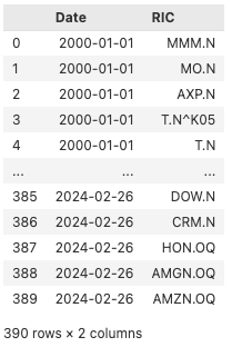
index_historical = ic.get_historical_constituents(index_ric, start = start_date, end=end_date)
index_historical
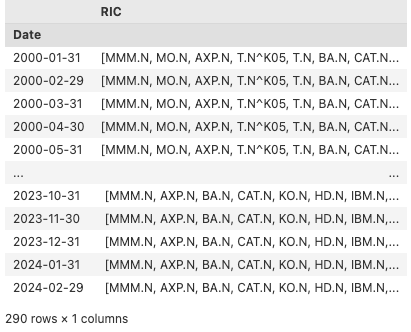
After obtaining the historical constituents for the DJI, we group the dataset by date, aggregate the RICs into a list, and resample monthly across the entire period in the dataset.
index_historical.set_index('Date', inplace=True)
index_historical.index = pd.to_datetime(index_historical.index)
index_grouped = index_historical.groupby('Date')['RIC'].agg(list)
ftse_grouped_m = pd.DataFrame(index_grouped.resample('M', convention='start').ffill())
ftse_grouped_m
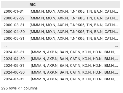
Since the last change to the constituents happened on February 2024, we can extend the RIC list of the last month for the rest of the observation period (July 2024).
last_date = ftse_grouped_m.index[-1]
last_constituents = ftse_grouped_m.iloc[-1]['RIC']
extended_dates = pd.date_range(start='2024-03-31', end='2024-07-31', freq='M')
extended_rows = pd.DataFrame({'RIC': [last_constituents] * len(extended_dates)}, index=extended_dates)
ftse_grouped_m = pd.concat([ftse_grouped_m, extended_rows])
ftse_grouped_m
Below, we define all the fields required for factor calculation. We have also included comments indicating which factors utilize each field. It should be noted that some fields are used across multiple factor calculations, for example, although "TR.CompanyMarketCap" is mentioned under size it is part of the formulas to be used for calculating Value factor.
fields = [
"TR.TRBCEconomicSector",
# Momentum
"TR.TotalReturn1Mo",
"TR.TotalReturn52Wk",
# Profitability
"TR.F.AssetTurnover(Period=FY0)",
"TR.F.AssetTurnover(Period=FY-1)",
"TR.F.ReturnAvgTotAssetsPct(Period=FY0)",
"TR.F.TotAssets(Period=FY0)",
"TR.F.TotAssets(Period=FY-1)",
"TR.F.WkgCap(Period=FY0)",
"TR.F.WkgCap(Period=FY-1)",
"TR.F.TotCurrAssets(Period=FY0)",
"TR.F.TotCurrAssets(Period=FY-1)",
"TR.F.InvstTot(Period=FY0)",
"TR.F.InvstTot(Period=FY-1)",
"TR.F.CustAdvTot(Period=FY0)",
"TR.F.CustAdvTot(Period=FY-1)",
"TR.F.TotLiab(Period=FY0)",
"TR.F.TotLiab(Period=FY-1)",
"TR.F.TotCurrLiab(Period=FY0)",
"TR.F.TotCurrLiab(Period=FY-1)",
"TR.F.PrefStockLiabPortLT(Period=FY0)",
"TR.F.PrefStockLiabPortLT(Period=FY-1)",
"TR.F.CashSTInvst(Period=FY0)",
"TR.F.CashSTInvst(Period=FY-1)",
"TR.F.InvstLT(Period=FY0)",
"TR.F.InvstLT(Period=FY-1)",
# Leverage
"TR.F.NetCashFlowOp(Period=FY0)",
"TR.F.NetCashFlowOp(Period=FY-1)",
"TR.F.DebtTot(Period=FY0)",
"TR.F.DebtTot(Period=FY-1)",
"TR.F.DebtLTTot(Period=FY0)",
"TR.F.DebtLTTot(Period=FY-1)",
# Size
"TR.CompanyMarketCap",
#Value
"TR.F.CF(Period=FY0)",
"TR.NetIncome(Period=FY0)",
"TR.Revenue(Period=FY0)",
#Yield
'TR.DividendYield'
]
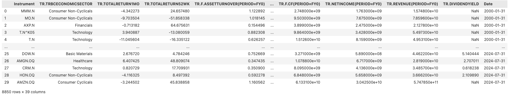
After we have our fields defined, we proceed with requesting the financial data using get_data function from LD libraries. Since we will be sending multiple requests to the API, it is always advisable to wrap the call in try/except statements to catch any occasional communication errors and retry the call. Additionally, we utilize header_type parameter of the function and set it to be the NAME (default value being TITLE) of the field since we request same fields with different fiscal periods.
max_steps = 5
dataset = pd.DataFrame()
for row in ftse_grouped_m.itertuples():
step = 0
while step < max_steps:
print(row.Index.date())
try:
df = ld.get_data(row.RIC, fields=fields, parameters={'SDate': f'{row.Index.date()}'}, header_type=HeaderType.NAME)
df['Date'] = row.Index.date()
dataset = pd.concat([dataset, df])
break
except errors.LDError as e:
print("LDError message:", e.message)
step +=1
time.sleep(5)
continue
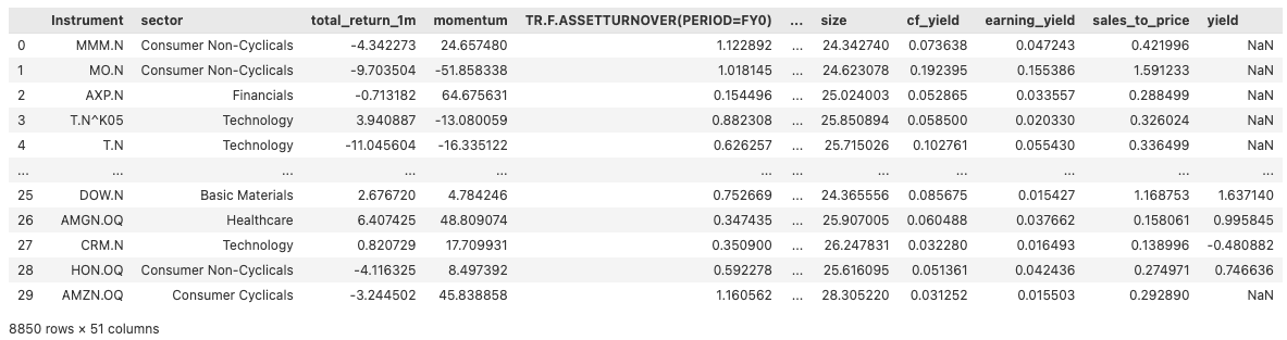
dataset
Building the factors
Calculating factor constituents
Before calculating the actual factor values, we first calculate their components, for example profitability is comprised of Return on Asset (roa), Change in Asset Turnover (at_delta) and accruals(accruals). More about the factor components and the formulas can be found in FTSE Global Factor Index Series Ground Rules.
dataset['at_delta'] = dataset['TR.F.ASSETTURNOVER(PERIOD=FY0)'] - dataset['TR.F.ASSETTURNOVER(PERIOD=FY-1)']
dataset['wk_delta'] = dataset['TR.F.WKGCAP(PERIOD=FY0)'] = dataset['TR.F.WKGCAP(PERIOD=FY-1)']
dataset['nco_delta'] = ((dataset['TR.F.TOTASSETS(PERIOD=FY0)'] - dataset['TR.F.TOTCURRASSETS(PERIOD=FY0)'] - dataset['TR.F.INVSTTOT(PERIOD=FY0)']) - (dataset['TR.F.TOTLIAB(PERIOD=FY0)'] - dataset['TR.F.TOTCURRLIAB(PERIOD=FY0)'] - dataset['TR.F.DEBTLTTOT(PERIOD=FY0)'])) - \
((dataset['TR.F.TOTASSETS(PERIOD=FY-1)'] - dataset['TR.F.TOTCURRASSETS(PERIOD=FY-1)'] - dataset['TR.F.INVSTTOT(PERIOD=FY-1)']) - (dataset['TR.F.TOTLIAB(PERIOD=FY-1)'] - dataset['TR.F.TOTCURRLIAB(PERIOD=FY-1)'] - dataset['TR.F.DEBTLTTOT(PERIOD=FY-1)']))
dataset['fin_delta'] = (dataset['TR.F.INVSTTOT(PERIOD=FY0)'] - dataset['TR.F.DEBTTOT(PERIOD=FY0)']) - (dataset['TR.F.INVSTTOT(PERIOD=FY-1)'] - dataset['TR.F.DEBTTOT(PERIOD=FY-1)'])
dataset['average_ta'] = (dataset['TR.F.TOTASSETS(PERIOD=FY0)'] + dataset['TR.F.TOTASSETS(PERIOD=FY0)'])/2
dataset['accruals'] = -(dataset['wk_delta']+dataset['nco_delta'] + dataset['fin_delta'])/dataset['average_ta']
dataset['leverage'] = dataset['TR.F.NETCASHFLOWOP(PERIOD=FY0)']/dataset['TR.F.DEBTTOT(PERIOD=FY0)']
dataset['size'] = np.log(dataset['TR.COMPANYMARKETCAP'])
dataset['cf_yield'] = dataset['TR.F.CF(PERIOD=FY0)']/dataset['TR.COMPANYMARKETCAP']
dataset['earning_yield'] = dataset['TR.NETINCOME(PERIOD=FY0)']/dataset['TR.COMPANYMARKETCAP']
dataset['sales_to_price'] = dataset['TR.REVENUE(PERIOD=FY0)']/dataset['TR.COMPANYMARKETCAP']
dataset['TR.DIVIDENDYIELD'] = pd.to_numeric(dataset['TR.DIVIDENDYIELD'], errors='coerce')
dataset['yield'] = np.log(dataset['TR.DIVIDENDYIELD'])
dataset.rename(columns={'TR.TOTALRETURN1MO': 'total_return_1m',
'TR.TOTALRETURN52WK': 'momentum',
'TR.F.RETURNAVGTOTASSETSPCT(PERIOD=FY0)': 'roa',
'TR.TRBCECONOMICSECTOR': 'sector'}, inplace=True)
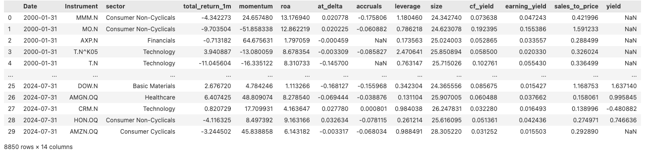
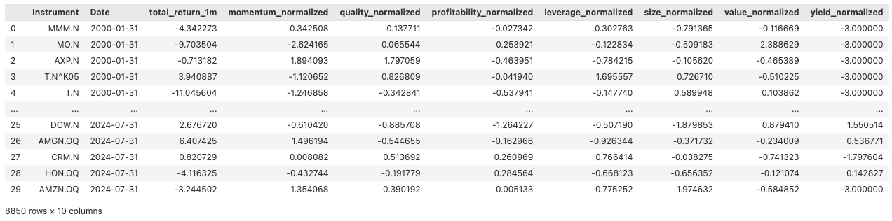
dataset
Next, we select only the factor components and apply data transformations, such as replacing inf with nan and making sure all number fields are numeric. This step is necessary for downstream feature normalization.
factor_components = ['Date', 'Instrument', 'sector', 'total_return_1m', 'momentum', 'roa', 'at_delta', 'accruals', 'leverage', 'size', 'cf_yield', 'earning_yield', 'sales_to_price', 'yield']
df_factor_components = dataset[factor_components]
df_factor_components.replace([np.inf, -np.inf], np.nan, inplace=True)
for col in factor_components[3:]:
df_factor_components[col] = pd.to_numeric(df_factor_components[col], errors='coerce').astype('float64')
df_factor_components
After, we normalize the ratios using StandardScaler (which uses z-score), smooth outliers out by clipping values and re-normalize in the range [-3, 3]. Again, the methodology is coming from FTSE Global Factor Index Series Ground Rules. For ease of use, we encapsulated normalization and outlier handling functions into separate functions:
def handle_outliers(series: np.ndarray, scaler:StandardScaler) -> np.ndarray:
#define the condition
condition = np.any((series > 3) | (series < -3))
# Handles outliers by clipping values and re-normalizing until within the condition range
while condition:
series = np.clip(series, -3, 3)
series = scaler.fit_transform(series)
condition = np.any((series > 3) | (series < -3))
return series
def normalize_factors(df: pd.DataFrame, factor_columns: list) -> pd.DataFrame:
scaler = StandardScaler()
df_norm = pd.DataFrame()
# Iterate over each unique date to normalize factor columns
for date in df['Date'].unique():
date_df = df[df['Date'] == date]
# Normalize each specified factor column and handle outliers
for col in factor_columns:
normalized_series = scaler.fit_transform(np.array(date_df[col]).reshape(-1, 1))
normalized_series = handle_outliers(normalized_series, scaler)
date_df[f"{col}_normalized"] = normalized_series
# Combine normalized data back into a single DataFrame
df_norm = pd.concat([df_norm, date_df])
return df_norm
df_factor_components_norm = normalize_factors(df_factor_components, factor_components[4:])
df_factor_components_norm['profitability_normalized'] = df_factor_components_norm[['roa_normalized', 'at_delta_normalized', 'accruals_normalized']].mean(axis=1, skipna=True)
df_factor_components_norm['quality_normalized'] = np.where(df_factor_components_norm['sector'] == 'Financials', df_factor_components_norm['roa'],
df_factor_components_norm[['profitability_normalized', 'leverage_normalized']].mean(axis=1, skipna=True))
df_factor_components_norm['value_normalized'] = df_factor_components_norm[['cf_yield_normalized', 'earning_yield_normalized', 'sales_to_price_normalized']].mean(axis=1, skipna=True)
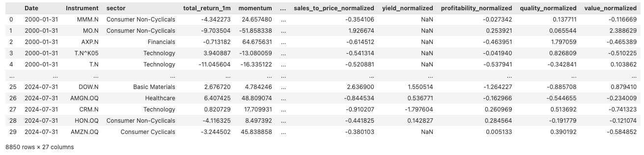
df_factor_components_norm
Finally, we keep only the final factor columns from our dataset.
factor_cols = ['momentum_normalized','quality_normalized', 'profitability_normalized', 'leverage_normalized', 'size_normalized', 'value_normalized', 'yield_normalized']
df_factors = df_factor_components_norm[['Instrument', 'Date', 'total_return_1m'] + factor_cols]
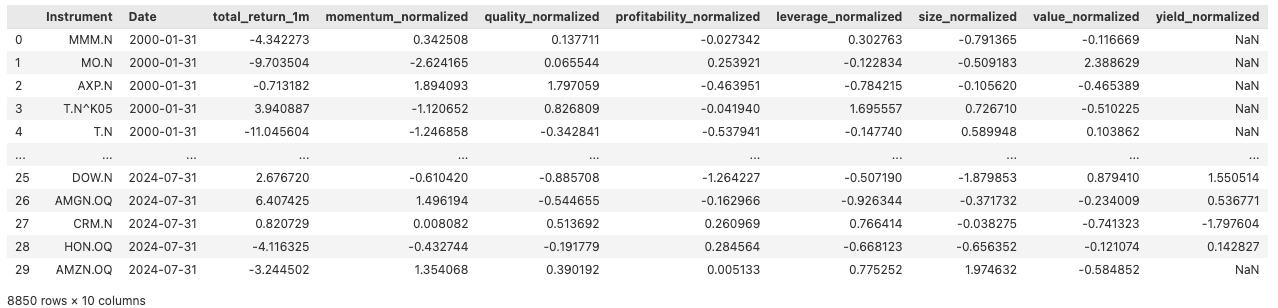
df_factors
One last step before we finalise the factor dataset is to handle the missing values. Following the FTSE Ground rules, for all factors with the exception of yield, stocks with missing factor data are allocated a neutral Z-score of 0 after the normalisation procedure. For Yield missing values are assigned a Z-score of -3.
for col in factor_cols:
if col == 'yield_normalized':
df_factors[col].fillna(-3, inplace=True)
else:
df_factors[col].fillna(0, inplace=True)
df_factors
Factor-Based Weighting
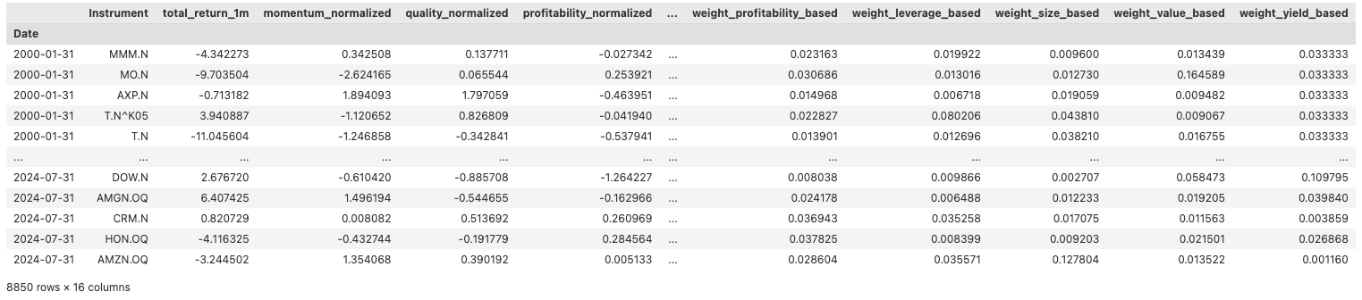
After we acquire the normalized factor values, we proceed by defining a function to calculate weights for each stock across all factors for every month. This function, when systematically applied generates new columns that contain the calculated weights for each stock per month, corresponding to each factor.
def get_factor_based_weights(series: pd.Series) -> pd.Series:
return np.exp(series) / np.sum(np.exp(series))
df_factors_and_weights = pd.DataFrame()
for date in df_factors['Date'].unique():
date_df = df_factors[df_factors['Date'] == date]
for factor in factor_cols:
factor_based_weights = get_factor_based_weights(date_df[factor])
date_df[f"weight_{factor.split('_')[0]}_based"] = factor_based_weights
df_factors_and_weights = pd.concat([df_factors_and_weights, date_df])
df_factors_and_weights.set_index('Date', inplace=True)
df_factors_and_weights
Building the feature set
Factor-based features
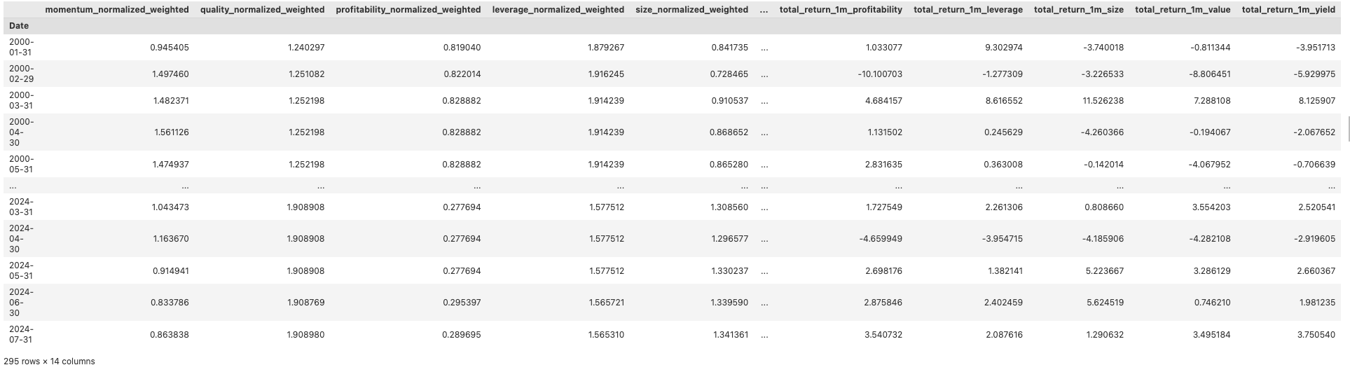
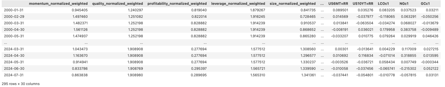
To create our factor-based feature set, we first compute weighted values for each factor by multiplying with its corresponding weight. Additionally, we calculate the weighted 1-month returns by multiplying the total 1-month return by the same factor weights. Finally, we aggregate these weighted values and returns by month, summing them up to produce a consolidated dataset. This aggregation results in a new DataFrame, where each column represents the summed weighted values and returns for each factor, grouped by date.
factors = df_factors_and_weights.columns[2:9]
weights = df_factors_and_weights.columns[9:]
for factor, weight in zip(factors, weights):
df_factors_and_weights[f'{factor}_weighted'] = df_factors_and_weights[factor] * df_factors_and_weights[weight]
df_factors_and_weights[f'total_return_1m_{factor.split("_")[0]}'] = df_factors_and_weights['total_return_1m'] * df_factors_and_weights[weight]
new_columns_factors = [f'{factor}_weighted' for factor in factors]
new_columns_returns = [f'total_return_1m_{factor.split("_")[0]}' for factor in factors]
feature_df = df_factors_and_weights[new_columns_factors + new_columns_returns].groupby(df_factors_and_weights.index).sum()
feature_df
Macro economic features
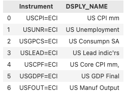
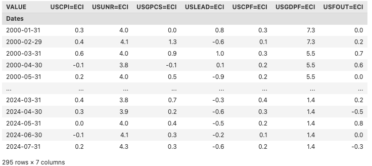
Macro economic indicators, such as GDP growth, unemployment rates, inflation etc, are important indicators that reflect the overall health of the economy. As different factors perform better under varying economic conditions, we are using a set of those indicators as initial features for our model. Below, we define some of those for the US which we believe is a good starting point. The full list of macroeconomic indicators can be found in ECONOMIND app in LSEG Workspace.
macro_rics = [
'USCPI=ECI',
'USUNR=ECI',
'USGPCS=ECI',
'USLEAD=ECI',
'USCPF=ECI',
'USGDPF=ECI',
'USFOUT=ECI',
]
macro_ind_names = ld.get_data(macro_rics, fields=['DSPLY_NAME'])
macro_ind_names
We also request historical data for the fields above covering our observation period. Additionally, we use a function to align dates with our feature dataframe (feature_df) for subsequent merging.
def allign_dates(ind_df: pd.DataFrame, df_to_allign_with:pd.DataFrame)->pd.DataFrame:
ind_df.columns = ind_df.columns.get_level_values(0)
ind_df['Dates'] = df_to_allign_with.index
ind_df.set_index('Dates', inplace=True)
return ind_df
start_date_macro = pd.to_datetime(start_date) - timedelta(days=30)
macro = ld.get_history(macro_rics, start=start_date_macro, end=end_date).ffill()[1:]
macro = allign_dates(macro, feature_df)
macro
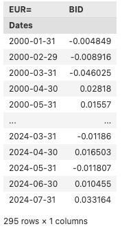
Currency feature
Currency fluctuations impact international trade and the earnings of companies with global exposure, therefore currency is another factor we have considered for the model. In this research we will be looking into the EURUSD pair.
curs = ['EUR=']
cur_prices = ld.get_history(curs, fields='BID', start=start_date, end='2024-08-31', interval='monthly')
cur_prices_change = cur_prices.pct_change().dropna()
cur_prices_change = allign_dates(cur_prices_change, feature_df)
cur_prices_change
Market indices features
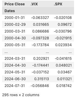
Another set of factors we believe can impact the factor performance are the market indicators, such as S&P 500(SPX) and the Volatility index(VIX).The SPX performance and VIX together capture market sentiment and volatility. In bull markets with low volatility, momentum and size factors may often outperform. During high volatility or bear markets, value, quality, and yield factors become more attractive as investment mediums.
ind = ['.VIX', '.SPX']
ind_prices = ld.get_history(ind, fields=["TR.PriceClose"], start='2000-01-01', end='2024-08-31', interval='monthly')
ind_prices_change = ind_prices.pct_change().dropna()
ind_prices_change = allign_dates(ind_prices_change, feature_df)
ind_prices_change
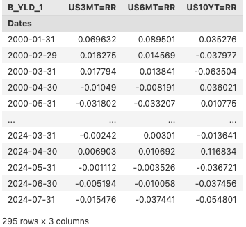
Bond features
Bond yields reflect interest rate expectations and risk sentiment. Rising yields might indicate stronger economic growth expectations, potentially favouring size or momentum factors. On the other hand, falling yields often signal risk aversion or economic slowdown, which might benefit more passive factors such as quality or value. We will be using 3M, 6M and 10Y bonds prices as a proxy for bond market.
bonds = ['US3MT=RR', 'US6MT=RR', 'US10YT=RR']
start_date_bonds = pd.to_datetime(start_date) - timedelta(days=30)
bonds_prices = ld.get_history(bonds, fields=["B_YLD_1"], start=start_date_bonds, end=end_date, interval='monthly')
bonds_prices_change = bonds_prices.pct_change().dropna()
bonds_prices_change = allign_dates(bonds_prices_change, feature_df)
bonds_prices_change
Commodity features
Commodity features, such as futures prices for oil, gas and gold are the final set of features have considered for the model as those prices directly affect certain sectors (e.g., energy, materials) and the broader economy.
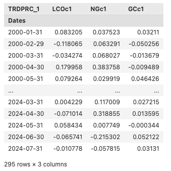
comods = ['LCOc1', 'NGc1', 'GCc1']
comods_prices = ld.get_history(comods, fields=["TRDPRC_1"], start='2000-01-01', end='2024-08-31', interval='monthly')
comods_prices_change = comods_prices.pct_change().dropna()
comods_prices_change = allign_dates(comods_prices_change, feature_df)
comods_prices_change
model_df = pd.concat([feature_df, macro, ind_prices_change, cur_prices_change, bonds_prices_change, comods_prices_change], axis = 1)
model_df
Creating the target variable
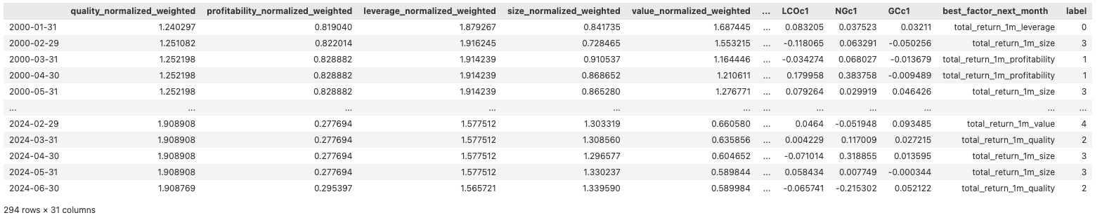
Our target variable, best_factor_next_month is created by taking the factor with the highest 1-month total return.
model_df['best_factor_next_month'] = model_df[[
'total_return_1m_momentum',
'total_return_1m_quality',
'total_return_1m_profitability',
'total_return_1m_leverage',
'total_return_1m_size',
'total_return_1m_value',
'total_return_1m_yield'
]].shift(-1).idxmax(axis=1)
for row in model_df['best_factor_next_month'].unique():
print(row, len(model_df[model_df['best_factor_next_month'] == row]))
total_return_1m_momentum 132
total_return_1m_size 34
total_return_1m_profitability 16
total_return_1m_value 20
total_return_1m_leverage 46
total_return_1m_yield 18
total_return_1m_quality 28
nan 0
Examining the distribution of label classes, we observe some data imbalance, skewed towards the momentum factor. This imbalance may bias our model towards the momentum class, limiting its ability to generalize across other factors. To address this and to focus on the underrepresented yet critical factors, we have decided to remove the momentum factor from our analysis. This approach is intended to help the model more effectively learn patterns related to these other factors, potentially improving overall performance. While techniques like oversampling, undersampling etc could be used to mitigate class imbalance, in the context of this study, we opted for a simpler approach as our primary goal here is to demonstrate whether factor-based index rebalancing can enhance performance compared to the base index.
model_df['best_factor_next_month'] = model_df[[
'total_return_1m_quality',
'total_return_1m_profitability',
'total_return_1m_leverage',
'total_return_1m_size',
'total_return_1m_value',
'total_return_1m_yield'
]].shift(-1).idxmax(axis=1)
# since we drop the momentum class, we will also drop the momentum feature
model_df = model_df.drop(columns=['momentum_normalized_weighted'])
model_df.dropna(inplace=True, subset=['best_factor_next_month'])
for row in model_df['best_factor_next_month'].unique():
print(row, len(model_df[model_df['best_factor_next_month'] == row]))
total_return_1m_leverage 75
total_return_1m_size 69
total_return_1m_profitability 37
total_return_1m_yield 35
total_return_1m_value 31
total_return_1m_quality 47
We use LabelEncoder to transform the remaining labels.
label_encoder = LabelEncoder()
model_df['label'] = label_encoder.fit_transform(model_df['best_factor_next_month'])
model_df
After removing the momentum factor, the distribution of the remaining factors shows a more balanced representation, though some imbalance persists, particularly between leverage and value. To address the slight remaining imbalance and ensure robust performance across all factors, we will employ XGBoost with sample weights, allowing the model to account for the distribution differences in class representation.
To get our initial list of features we should exclude all total return columns which we used for creating the label.
features = [col for col in model_df.columns[:-2] if not col.startswith("total")]
print(len(features))
22
Recursive Feature Elimination
As demonstrated above, we have a total of 22 features, and given our dataset of 290 observations, it is important to eliminate some features to reduce model complexity and minimize the risk of overfitting. To achieve this, we implement recursive feature elimination, a feature selection strategy using XGBoost. By applying this methodology, we iteratively rank the features based on their importance to the model's predictions and systematically remove the least significant ones. This process continues until the top 12 features remain. We retain 12 features as it allows around 20 observations (train set is around 230 observations) per feature which is a good rule of thumb for ensemble models. This approach allows us to maintain the most critical features that contribute to the model's predictive accuracy, reduce the complexity of the model and minimize the risk of overfitting.
Before implementing feature elimination, we split our dataset into training and test sets. Observations prior to January 2019 are assigned to the training set, while those from January 2019 onward are reserved for the test set. We opt for a temporal train/test split instead of a random split because maintaining the chronological order of observations is essential for testing the investment performance of our rebalancing approach.
scaler = StandardScaler()
split_idx = model_df[model_df.index < '2019-01-01'].shape[0]
y_encoded = (model_df['best_factor_next_month'])
X_train, X_test, y_train, y_test = model_df[:split_idx][features], model_df[split_idx:][features], model_df['label'][:split_idx], model_df['label'][split_idx:]
X_train_norm = pd.DataFrame(scaler.fit_transform(X_train), columns=X_train.columns)
As mentioned above, we train the model with sample weights to address label imbalancing using the function below.
def calculate_sample_weights(y_train):
class_counts = np.bincount(y_train)
total_samples = len(y_train)
class_weights = total_samples / (len(np.unique(y_train)) * class_counts)
sample_weights = np.array([class_weights[class_index] for class_index in y_train])
return sample_weights
Below, we implement the recursive feature selection as described above and show the 12 most important features along with the importance scores.
model = xgb.XGBClassifier(random_state = 42)
features = X_train_norm.columns.tolist()
n_features_to_select = 12
sample_weights = calculate_sample_weights(y_train)
while len(features) > n_features_to_select:
model.fit(X_train_norm[features], y_train, sample_weight=sample_weights)
importances = model.feature_importances_
least_important = np.argmin(importances)
features.pop(least_important)
important_features_df = pd.DataFrame({
'Feature': features,
'Importance': importances[:-1]
})
important_features_df = important_features_df.sort_values(by=['Importance'], ascending=False).reset_index(drop=True)
important_features_df
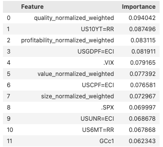
The most important features include a mix of economic, bond, and market, as well as factor-based indicators which is demonstrating a balanced selection of features which we will use for rolling training window and out of sample testing.
X_train, X_test = model_df[:split_idx][important_features_df['Feature']], model_df[split_idx:][important_features_df['Feature']]
X_train_norm = pd.DataFrame(scaler.fit_transform(X_train), columns=X_train.columns)
Rolling Training window and performance results
Out of sample testing
Below, we define a function to train the model which uses XgBoost with softprob objective (allowing to return probabilities along with the predictions), cross entropy loss and fits the model using sample weights. For simplicity, we didn't implement any hyperparameter tuning, which could potentially further enhance the model's predictive power.
def train_model(X_train_norm, y_train):
sample_weights = calculate_sample_weights(y_train)
model = xgb.XGBClassifier(
objective='multi:softprob',
num_class=len(np.unique(y_train)),
use_label_encoder=False,
eval_metric='mlogloss',
random_state = 42)
model.fit(X_train_norm, y_train, sample_weight=sample_weights)
return model
The rolling training window process is implemented in two steps: first, we train an initial model using the training dataset consisting of observations up to January 2019. Then, we predict the factor for the following month, add this new observation to the training set, retrain the model, and predict the next month. This process is repeated for all test observations after January 2019. In addition to the actual predictions, we store the prediction probabilities, which will be used to build a probabilistic investment strategy.
# initial training
predictions = []
predict_proba = []
model = train_model(X_train_norm, y_train)
# rolling training and out of sample testing
for sample, y in zip(X_test.iterrows(), y_test):
sample = scaler.transform(pd.DataFrame(sample[1]).T)
predictions.append(model.predict(sample)[0])
predict_proba.append(model.predict_proba(sample))
X_train_norm = np.concatenate((X_train_norm, sample))
y_train = np.concatenate((y_train, np.array([y])))
model = train_model(X_train_norm, y_train)
label_mapping = dict(zip(model_df['label'], model_df['best_factor_next_month']))
target_names = [label_mapping[i] for i in sorted(model_df['label'].unique())]
report = classification_report(y_test, predictions,
target_names=target_names
)
print(f"Actual Prediction:\n {dict(sorted(Counter(predictions).items()))} \n")
print(f"Confusion Matrix:\n {confusion_matrix(y_test, predictions)}\n")
print("Classification Report:\n", report)
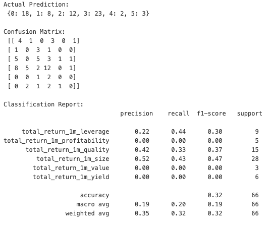
Although the model's accuracy is 32% for the 6-class classification task, accuracy alone may not fully capture the model's effectiveness in context. Our main goal is to compare index performance with and without prediction-based factor rebalancing. Even if the model doesn't consistently identify the top-performing factor, choosing the next best factor can still enhance performance compared to the base factor (e.g., the DJI, which is price-weighted). The confusion matrix highlights that the model performs best in identifying the leverage, quality and size factors, with 4 and 5 and 12 correct predictions accordingly, while struggling most with the yield, profitability and value classes, where misclassifications were more frequent.
Given our objective, a more suitable metric to consider might be the Top-N Accuracy, which focuses on how often the model's top predictions include the actual correct factor, rather than just its first choice. These metrics are more aligned with our goal of improving index performance through factor rebalancing, where correctly identifying one of the top factors, even if not the very best one, can be beneficial.
We use top_n_accuracy function to calculate the accuracy of correctly predicting one of the top 3 classes.
def top_n_accuracy(y_true, y_pred_proba, n=3):
y_pred_proba = np.vstack(y_pred_proba)
top_n_pred = np.argsort(y_pred_proba, axis=1)[:, -n:]
matches = [y_true[i] in top_n_pred[i] for i in range(len(y_true))]
return np.mean(matches)
top_3_acc = top_n_accuracy(y_test, predict_proba, n=3)
print("top-3 accuracy:", top_3_acc)
top-3 accuracy: 0.6212121212121212
The model achieved a 62% Top-3 accuracy, indicating that its predictions included the correct factor within the top 3 for 62% of the test observations. Nevertheless, the most effective way to assess the model's performance is by applying the rebalancing strategy based on these predictions and comparing the rebalanced index's performance with the actual index performance.
Index rebalancing performance comparison
We will introduce and compare two rebalancing strategies against the main DJI index:
- Rebalancing based on the Top Prediction: In this strategy, the index will be rebalanced based on the top predicted factor. For example, if the model predicts size as the best factor, the index will be rebalanced using returns derived from size-based weights.
- Weighted rebalancing based on prediction probabilities: In this approach, the index will be rebalanced by calculating a weighted sum of returns, where each factor's return is weighted by its predicted probability.
Adding predictions
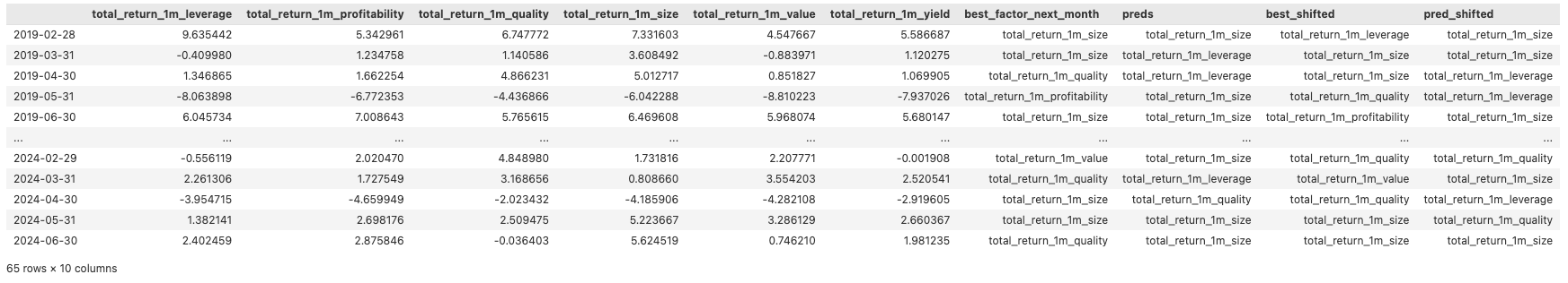
To start with, we create a new dataframe representing the return columns and the best factor names for the test period. Then we add the predictions and shift both the predictions and actual values by 1 period which aligns the predictions with the returns for the month. This is to ensure we are using the prediction or best factor from the previous month to calculate the return for the current month.
returns_df = model_df[target_names + ['best_factor_next_month']][split_idx:]
returns_df['preds'] = label_encoder.inverse_transform(predictions)
returns_df['best_shifted'] = returns_df['best_factor_next_month'].shift(1)
returns_df['pred_shifted'] = returns_df['preds'].shift(1)
returns_df = returns_df.dropna()
returns_df
Calculating prediction based returns
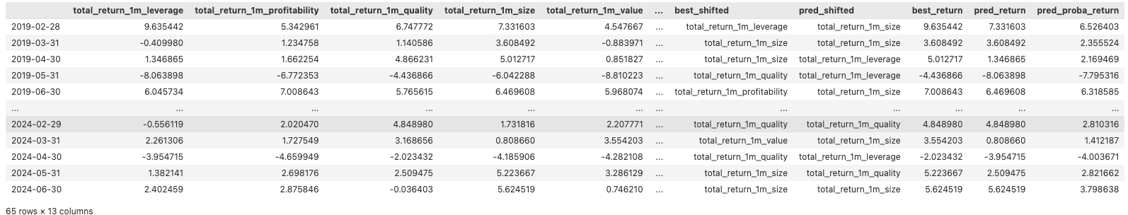
Next, we calculate 3 types of returns:
- best_return - the return if we always predicted the correct class
- pred_return - the return based on predicted factor
- pred_proba_return - weighted return based on prediction probabilities for each factor.
We use add_names_to_probas function to add the target names to the prediction probabilities and calculate_weighted_return for pred_proba_return calculaton.
def add_names_to_probas(target_names: list, predict_proba:list)->list:
proba_list = []
for probas in predict_proba:
probas_named = {}
for name, value in zip(target_names, probas[0]):
probas_named[name] = value
proba_list.append(probas_named)
return proba_list
def calculate_weighted_return(row:pd.DataFrame, probas:dict)->float:
return (probas['total_return_1m_leverage'] * row.total_return_1m_leverage +
probas['total_return_1m_profitability'] * row.total_return_1m_profitability +
probas['total_return_1m_quality'] * row.total_return_1m_quality +
probas['total_return_1m_size'] * row.total_return_1m_size +
probas['total_return_1m_value'] * row.total_return_1m_value +
probas['total_return_1m_yield'] * row.total_return_1m_yield)
returns_df['best_return'] = [ret[ret['best_shifted']] for _, ret in returns_df.iterrows()]
returns_df['pred_return'] = [ret[ret['pred_shifted']] for _, ret in returns_df.iterrows()]
returns_df['pred_proba_return'] = [
calculate_weighted_return(row, probas) for row, probas in zip(returns_df.itertuples(), add_names_to_probas(target_names, predict_proba))
]
returns_df
Calculating base index returns
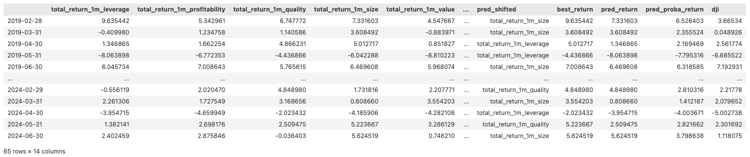
Below, we calculate returns for the base index and add to our returns dataframe.
dji = ld.get_history('.DJI', "TR.PriceClose", start='2019-01-31', end='2024-07-01', interval='monthly')
dji_change = dji.pct_change().dropna()
dji_change = allign_dates(dji_change, returns_df)
returns_df['dji'] = dji_change['Price Close']*100
returns_df
Additionally, we also calculate the cumulative returns.
cols_for_cumsum = target_names + ['best_return','pred_return','pred_proba_return', 'dji']
for col in cols_for_cumsum:
returns_df[f'{col}_cumsum'] = returns_df[col].cumsum()
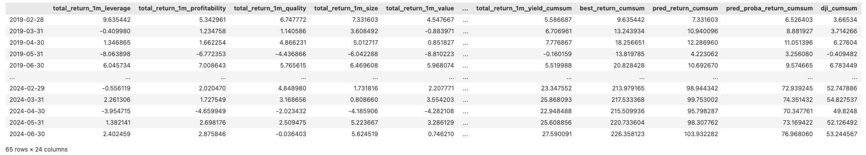
returns_df
Finally, we calculate the sharp ratio for the strategies and present the performance comparison in a separate dataframe.
def calculate_sharpe_ratio(returns:pd.Series, risk_free_rate: float =0) -> float:
excess_returns = returns - risk_free_rate
mean_excess_return = excess_returns.mean() * 100
std_excess_return = excess_returns.std() * 100
sharpe_ratio = mean_excess_return / std_excess_return
annualized_sharpe_ratio = sharpe_ratio * np.sqrt(252)
return annualized_sharpe_ratio
sharp_ratio = {}
cum_return = {}
for col in cols_for_cumsum:
cum_return[col] = returns_df[f"{col}_cumsum"][-1]
sharp_ratio[col] = calculate_sharpe_ratio(returns_df[col])
pd.DataFrame({'cum_return': cum_return, 'sharp_ratio': sharp_ratio}).sort_values(by=['cum_return'], ascending=False)
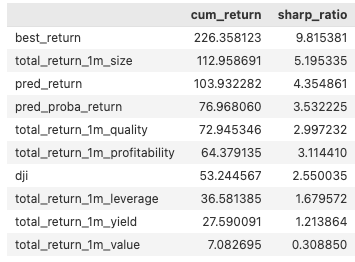
The "best_return" represents the theoretical maximum potential with a cumulative return of 226.36% and a Sharpe ratio of 9.82. Model-driven strategies, particularly "pred_return" and "pred_proba_return," outperformed the traditional benchmark. The "pred_return" achieved a cumulative return of 103.93% and a Sharpe ratio of 4.35, while "pred_proba_return" followed closely with a 76.96% return and a Sharpe ratio of 3.53. Both surpassed the base index, which had a cumulative return of 53.24% and a Sharpe ratio of 2.55. Factor-only strategies showed mixed results. The "total_return_1m_size" factor led with a 112.96% return and a Sharpe ratio of 5.20, while other factors, like "total_return_1m_value," significantly lagged, with just a 7.08% return and a Sharpe ratio of 0.31.
We also plot the cumulative returns for model-driven strategies and the base index.
fig = go.Figure()
for series_name in ['dji_cumsum', 'pred_return_cumsum', 'pred_proba_return_cumsum']:
fig.add_trace(go.Scatter(
x=returns_df.index,
y=returns_df[series_name],
mode='lines', name=series_name))
fig.show()
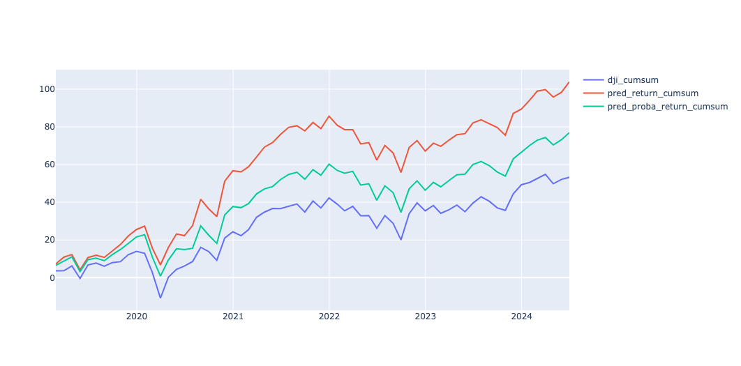
According to the plot, both model-driven strategies consistently outperformed the baseline throughout the observation period, with the prediction-based strategy outperforming the prediction-probability-based strategy demonstrating the added value of predictive modelling.
Conclusion
Our article demonstrated the process of retrieving historical index constituents, calculating associated financial ratios, and constructing factors to explore an advanced approach to index rebalancing that extends beyond traditional single-factor methodologies. The primary goal was to determine whether a multi-factor strategy, with dynamic adjustments based on predictions of the best-performing factors, could enhance the returns of a base index.
The results suggest that a multi-factor, model-driven approach to index rebalancing can outperform traditional single-factor indexes. By incorporating various financial and economic metrics and dynamically adjusting the index composition based on predicted factor performance, the model-driven strategies consistently achieved higher returns and better risk-adjusted outcomes. This showcases the potential of advanced rebalancing techniques to improve investment results.
However, it's important to note that this research is exploratory in nature. Further analysis is needed to ensure the robustness of the findings, including additional tests and validations. Hyperparameter tuning and sensitivity analysis could further refine the model's predictions and potentially enhance performance. Therefore, while the results are promising, they should be considered as a foundation for more comprehensive studies and practical applications.
- Register or Log in to applaud this article
- Let the author know how much this article helped you
Related Articles
-
Building historical index constituents
-
Modelling and Evaluation - Artificial Intelligence regression and classification performance metrics
-
Forward Looking Index Ratio Analysis
-
Market regime detection using Statistical and ML based approaches
-
Idiosyncratic risk ranking using eXplainable AI
-
Exploring AI Mentions in Earnings Calls and Building Thematic Portfolios
-
How to build an end-to-end transaction cost analysis framework