Author:


Code can be found on GitHub.
In this article, I exemplify how one may use pre-existing articles (such as Umer’s) together to form Jupyter Python Apps working alongside your Workspace Tiles environment using the Refinitiv Side by Side API.
1st, we will use Python functions created by Umer in his Instrument Pricing Analytics — Volatility Surfaces and Curves article to create FX Volatility Surfaces.
2nd, we will embed such graphs in a widget, using techniques shown in CodeBook examples (in ‘__ Examples __/04. Advanced UseCases/04.01. Python Apps/EX_04_01_02__WFCH_Company_Income_Statement_Waterfall.ipynb’) and online (shout out to ac24).
3rd, we will finally incorporate this workflow with the Refinitiv Side by Side API so that Tiles become linked with our notebook, reacting to them live (shout out to Evgeny Kovalyov).
In this article, we look at a simple example with an FX Quote Tile and Volatility Surfaces; but you are encouraged to use this code and work to create your own applications that work ergonomically with your workflow, whatever it may be. The techniques used below are very malleable and do not have to be used specifically for Volatility Surface creation. If you have an idea in mind and would like some help to code them up, don’t hesitate to submit your idea to the Article Competition and contact me.
Twitch Python Finance Webinar
Code
# Basic Python libraries:
import refinitiv.dataplatform as rdp
import ipywidgets as widgets
import pandas as pd
import IPython
from IPython.display import display, clear_output
# Python libraries needed specifically for Python:
import requests
from requests.exceptions import ConnectionError
import json
import functools
import enum
from enum import Enum
import time
import queue
import threading
import logging
import lomond
from lomond import WebSocket, events as websocket_events
from lomond.persist import persist
import typing
from typing import List, Tuple, Dict, Optional, Callable, Type, ClassVar, Any, Iterable
import sys # ' sys ' is a native Python library ('native' as in it does not need to be installed) that allows us to find details on the machine running the code and our Python version.
print("This code is running on Python version: " + sys.version) # This line shows us the details requiered.
for i, j in zip(["Refinitiv Data Platform", "ipywidgets", "pandas", "IPython", "requests", "json", "logging", "lomond"],
[rdp, widgets, pd, IPython, requests, json, logging, lomond]):
print(f"The imported {i} library is of version {j.__version__}")
This code is running on Python version: 3.8.2 (tags/v3.8.2:7b3ab59, Feb 25 2020, 22:45:29) [MSC v.1916 32 bit (Intel)]
The imported Refinitiv Data Platform library is of version 1.0.0a11.post1
The imported ipywidgets library is of version 7.6.3
The imported pandas library is of version 1.2.4
The imported IPython library is of version 7.22.0
The imported requests library is of version 2.23.0
The imported json library is of version 2.0.9
The imported logging library is of version 0.5.1.2
The imported lomond library is of version 0.3.3
Graph
As per the Instrument Pricing Analytics (Volatility Surfaces and Curves)'s notebook on GitHub, plotting_helper.ipynb, we need to:
1st: Authenticate ourselves to the Refinitiv Data Platform API:
# I store my login details on a .txt file that sits along side this notebook.
# The tree lines below (and the complementary .close() lines at the end of this cell) fetch these credentials for me.
# This way I can authenticate myself to RDP automatically and share my code without sharing my credentials.
APP_KEY = open("AppKey.txt", "r")
RDP_LOGIN = open("RdpLogin.txt", "r")
RDP_PASSWORD = open("RdpP.txt", "r")
session = rdp.DesktopSession( # You can try and use 'PlatformSession' instead of 'DesktopSession' if running Workspace/Eikon on your desktop in the background isn't an option, although that will negate the use of Tiles essential to this exercise.
APP_KEY.read(),
rdp.GrantPassword(username=RDP_LOGIN.read(),
password=RDP_PASSWORD.read()))
session.open()
APP_KEY.close()
RDP_LOGIN.close()
RDP_PASSWORD.close()
2nd: Now access the RDP endpoint we're interested in before sending a request and storing the response:
vs_endpoint = rdp.Endpoint(
session,
"https://api.edp.thomsonreuters.com/data/quantitative-analytics-curves-and-surfaces/v1/surfaces")
fx_request_body = {
"universe": [
{
"underlyingType": "Fx",
"surfaceTag": "FxVol-GBPUSD",
"underlyingDefinition": {
"fxCrossCode": "GBPUSD"
}, ...
},
{
"underlyingType": "Fx",
"surfaceTag": "FxVol-EURUSD",
"underlyingDefinition": {
"fxCrossCode": "EURUSD"
}, ...
},
{
"underlyingType": "Fx",
"surfaceTag": "FxVol-CHFUSD",
"underlyingDefinition": {
"fxCrossCode": "CHFUSD"
}, ... } ] }
fx_response = vs_endpoint.send_request(
method=rdp.Endpoint.RequestMethod.POST,
body_parameters=fx_request_body
)
# # If you wish to see the data imported, you can use the line below (comented out):
# print(json.dumps(fx_response.data.raw, indent=2))
The data above can take a while to be collected, you may want to keep it for multiple runs / debugging; I do so below using the Python library pickle:
# import pickle
# pickle_out = open("FxResp.pickle", "wb")
# pickle.dump(fx_response, pickle_out)
# pickle_out.close()
# # To load data in:
# pickle_in = open("FxResp.pickle","rb") # ' rb ' stand for 'read bytes'.
# fx_response = pickle.load(pickle_in)
# pickle_in.close() # We ought to close the file we opened to allow any other programs access if they need it.
3rd: Create functions to be used subsequentally in our code:
def convert_delta(delta):
if delta == 'ATM': return 0.5
elif delta < 0: return -delta
elif delta > 0: return 1-delta
else: return 0.5
# Convert float date back to Y-m-d for the Surface y axis tick labels
def format_date(x, pos=None):
import matplotlib.dates as dates
return dates.num2date(x).strftime('%Y-%m-%d') #use FuncFormatter to format dates
# Matplotlib requires dates in float format for surface plots.
def convert_yyyymmdd_to_float(date_string_array):
import datetime
import matplotlib.dates as dates
date_float_array = []
for date_string in date_string_array:
if len(date_string)==10:
date_float = dates.date2num(datetime.datetime.strptime(date_string, '%Y-%m-%d'))
else:
date_float = dates.date2num(datetime.datetime.strptime(date_string, '%Y-%m-%dT%H:%M:%SZ'))
date_float_array.append(date_float)
return date_float_array
def plot_surface(surfaces, surfaceTag, delta_plot=False):
# This import registers the 3D projection, but is otherwise unused.
from mpl_toolkits.mplot3d import Axes3D
import numpy as np
import matplotlib.pyplot as plt
from matplotlib import cm
import matplotlib.ticker as ticker # import LinearLocator, FormatStrFormatter
surfaces = pd.DataFrame(data=surfaces)
surfaces.set_index('surfaceTag', inplace=True)
surface = surfaces[surfaces.index == surfaceTag]['surface'][0]
strike_axis = surface[0][1:]
surface = surface[1:]
time_axis = []
surface_grid = []
for line in surface:
time_axis.append(line[0])
surface_grid_line = line[1:]
surface_grid.append(surface_grid_line)
time_axis = convert_yyyymmdd_to_float(time_axis)
if delta_plot:
# When plotting FX Delta rather than Strike
# I'm converting the x axis value from Delta to Put Delta
delta_axis = list(map(convert_delta, strike_axis))
x = np.array(delta_axis, dtype=float)
else:
x = np.array(strike_axis, dtype=float)
y = np.array(time_axis, dtype=float)
Z = np.array(surface_grid, dtype=float)
X, Y = np.meshgrid(x,y)
fig = plt.figure(figsize=[15, 10])
ax = plt.axes(projection='3d')
ax.set_facecolor('0.25')
ax.set_xlabel('Delta' if delta_plot else 'Moneyness', color='y', labelpad=10)
ax.set_ylabel('Expiry', color='y', labelpad=15)
ax.set_zlabel('Volatilities', color='y')
ax.tick_params(axis='both', colors='w')
ax.w_yaxis.set_major_formatter(ticker.FuncFormatter(format_date))
title = 'Vol Surface for : ' + str(surfaceTag)
ax.set_title(title, color='w')
surf = ax.plot_surface(X, Y, Z, cmap=cm.coolwarm, linewidth=0, antialiased=False)
plt.show()
Now let’s have a look at our retrieved data:
pd.DataFrame(fx_response.data.raw['data'][0]['surface'])
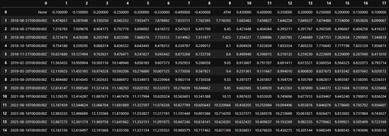
Notice that sometimes you may have a ATM value returned; this is something dealt with in our convert_delta function defined previously.
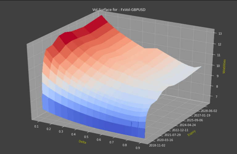
Now let’s plot our volatility surfaces:
fx_surfaces = fx_response.data.raw['data']
surfaces, surfaceTag, delta_plot = fx_surfaces, 'FxVol-CHFUSD', False
fx_surfaces = fx_response.data.raw['data']
plot_surface(fx_surfaces, 'FxVol-GBPUSD', True)
Widget
(Credit to ac24)
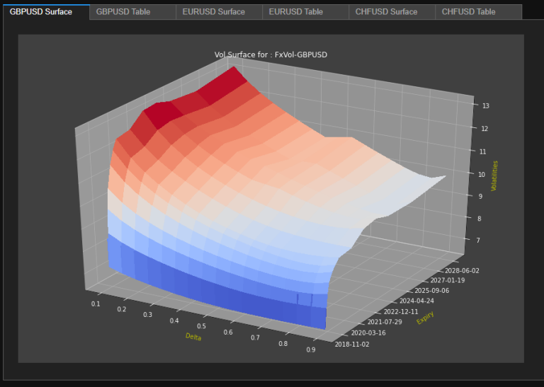
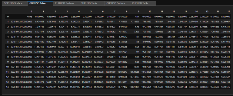
We can now look into incorporating our above graph in a widget that allows us to toggle between graph and data (in a table). This is a rudimentary example taken from CodeBook examples (in ‘__ Examples __/04. Advanced UseCases/04.01. Python Apps/EX_04_01_02__WFCH_Company_Income_Statement_Waterfall.ipynb’), but more complex ones can easily be constructed to fit your workflow.
%matplotlib inline
import ipywidgets as widgets
out1 = widgets.Output()
out2 = widgets.Output()
out3 = widgets.Output()
out4 = widgets.Output()
out5 = widgets.Output()
out6 = widgets.Output()
tab = widgets.Tab(children=[out1, out2, out3, out4, out5, out6])
tab.set_title(0, 'GBPUSD Surface')
tab.set_title(1, 'GBPUSD Table')
tab.set_title(2, 'EURUSD Surface')
tab.set_title(3, 'EURUSD Table')
tab.set_title(4, 'CHFUSD Surface')
tab.set_title(5, 'CHFUSD Table')
display(tab)
fx_surfaces = fx_response.data.raw['data']
surfaces = fx_surfaces
delta_plot = False
with out1:
fxplot = plot_surface(fx_surfaces, 'FxVol-GBPUSD', True)
with out2:
display(pd.DataFrame(fx_response.data.raw['data'][0]['surface']))
with out3:
fxplot = plot_surface(fx_surfaces, 'FxVol-EURUSD', True)
with out4:
display(pd.DataFrame(fx_response.data.raw['data'][1]['surface']))
with out5:
fxplot = plot_surface(fx_surfaces, 'FxVol-CHFUSD', True)
with out6:
display(pd.DataFrame(fx_response.data.raw['data'][2]['surface']))
Tab(children=(Output(), Output(), Output(), Output(), Output(), Output()), _titles={'0': 'GBPUSD Surface', '1'…
SxS
We’ll need to create functions to be used subsequently in our code:
There is a great deal of code here, see GitHub for code
And finally, we can launch a Quote Tile
launch('q') # using the code{'instance_id': '7bc1159a-412c-44be-b86a-435f88f8fd1f', 'h_wnd': 6949750}
You can play with the Tile and see the kind of information we receive:
# app_dict, app_dict_lst = get_app_list(), []
# while True:
# app_dict_lst.append(app_dict)
# time.sleep(3.0)
# app_dict = get_app_list()
# if app_dict != app_dict_lst[-1]:
# if len(app_dict['apps'][0]['name'].replace(' Quote', '')) != 4:
# display(app_dict['apps'][0]['name'].replace('= Quote', ''))
# elif app_dict['apps'][0]['name'].replace(' Quote', '') == 'Quote':
# pass
# else:
# display(app_dict['apps'][0]['name'].replace('= Quote', 'USD'))
# app_dict_lst = [app_dict_lst[-1]]
SxS & Widget
We’ll need to create functions to be used subsequently in our code:
def FxSxsWidget(
CurencyPair='EURGBP', calculationDate='2018-08-20T00:00:00Z',
APP_KEY='textFile', RDP_LOGIN='textFile', RDP_PASSWORD='textFile',
RdpEndpoint="https://api.edp.thomsonreuters.com/data/quantitative-analytics-curves-and-surfaces/v1/surfaces"):
# Basic Python libraries:
import refinitiv.dataplatform as rdp
import pandas as pd
# from datetime import datetime, timedelta
# # Python libraries needed specifically for Python:
# import requests
# from requests.exceptions import ConnectionError
# import json
# import functools
# from enum import Enum
# import time
# import queue
# import threading
# import logging
# from lomond import WebSocket, events as websocket_events
# from lomond.persist import persist
# from typing import List, Tuple, Dict, Optional, Callable, Type, ClassVar, Any, Iterable
## Making sure that the 'CurencyPair' argument is adequate and won't break our code:
if len(CurencyPair) == 4:
CurencyPair = CurencyPair.replace('=', 'USD')
## Define functions needed:
def convert_delta(delta):
if delta == 'ATM': return 0.5
elif delta < 0: return -delta
elif delta > 0: return 1-delta
else: return 0.5
# Convert float date back to Y-m-d for the Surface y axis tick labels
def format_date(x, pos=None):
import matplotlib.dates as dates
return dates.num2date(x).strftime('%Y-%m-%d') #use FuncFormatter to format dates
# Matplotlib requires dates in float format for surface plots.
def convert_yyyymmdd_to_float(date_string_array):
import datetime
import matplotlib.dates as dates
date_float_array = []
for date_string in date_string_array:
if len(date_string)==10:
date_float = dates.date2num(datetime.datetime.strptime(date_string, '%Y-%m-%d'))
else:
date_float = dates.date2num(datetime.datetime.strptime(date_string, '%Y-%m-%dT%H:%M:%SZ'))
date_float_array.append(date_float)
return date_float_array
def plot_surface(surfaces, surfaceTag, delta_plot=False):
# This import registers the 3D projection, but is otherwise unused.
from mpl_toolkits.mplot3d import Axes3D
import numpy as np
import matplotlib.pyplot as plt
from matplotlib import cm
import matplotlib.ticker as ticker # import LinearLocator, FormatStrFormatter
surfaces = pd.DataFrame(data=surfaces)
surfaces.set_index('surfaceTag', inplace=True)
surface = surfaces[surfaces.index == surfaceTag]['surface'][0]
strike_axis = surface[0][1:]
surface = surface[1:]
time_axis = []
surface_grid = []
for line in surface:
time_axis.append(line[0])
surface_grid_line = line[1:]
surface_grid.append(surface_grid_line)
time_axis = convert_yyyymmdd_to_float(time_axis)
if delta_plot:
# When plotting FX Delta rather than Strike
# I'm converting the x axis value from Delta to Put Delta
delta_axis = list(map(convert_delta, strike_axis))
x = np.array(delta_axis, dtype=float)
else:
x = np.array(strike_axis, dtype=float)
y = np.array(time_axis, dtype=float)
Z = np.array(surface_grid, dtype=float)
X, Y = np.meshgrid(x,y)
fig = plt.figure(figsize=[15, 10])
ax = plt.axes(projection='3d')
ax.set_facecolor('0.25')
ax.set_xlabel('Delta' if delta_plot else 'Moneyness', color='y', labelpad=10)
ax.set_ylabel('Expiry', color='y', labelpad=15)
ax.set_zlabel('Volatilities', color='y')
ax.tick_params(axis='both', colors='w')
ax.w_yaxis.set_major_formatter(ticker.FuncFormatter(format_date))
title = 'Vol Surface for : ' + str(surfaceTag)
ax.set_title(title, color='w')
surf = ax.plot_surface(X, Y, Z, cmap=cm.coolwarm, linewidth=0, antialiased=False)
plt.show()
## Authenticate ourselves to rdp
if APP_KEY=='textFile': APP_KEY = open("AppKey.txt", "r")
if RDP_LOGIN=='textFile': RDP_LOGIN = open("RdpLogin.txt", "r")
if RDP_PASSWORD=='textFile': RDP_PASSWORD = open("RdpP.txt", "r")
session = rdp.DesktopSession(# .PlatformSession
APP_KEY.read(),
rdp.GrantPassword(username=RDP_LOGIN.read(),
password=RDP_PASSWORD.read()))
session.open()
APP_KEY.close()
RDP_LOGIN.close()
RDP_PASSWORD.close()
## Choose correct rdp endpoint:
vs_endpoint = rdp.Endpoint(session, RdpEndpoint)
## Build body of data request and send it:
fx_request_body = {
"universe": [
{
"underlyingType": "Fx",
"surfaceTag": f"FxVol-{CurencyPair}",
"underlyingDefinition": {
"fxCrossCode": CurencyPair
},
"surfaceLayout": {
"format": "Matrix"
},
"surfaceParameters": {
"xAxis": "Date",
"yAxis": "Delta",
"calculationDate": calculationDate,
"returnAtm": "True"
}
}
]
}
fx_response = vs_endpoint.send_request(
method=rdp.Endpoint.RequestMethod.POST,
body_parameters=fx_request_body)
%matplotlib inline
import ipywidgets as widgets
out1, out2 = widgets.Output(), widgets.Output()
tab = widgets.Tab(children=[out1, out2])
tab.set_title(0, f"{CurencyPair} Surface")
tab.set_title(1, f"{CurencyPair} Table")
display(tab)
fx_surfaces = fx_response.data.raw['data']
surfaces, delta_plot = fx_surfaces, False
with out1:
fxplot = plot_surface(fx_surfaces, f"FxVol-{CurencyPair}", True)
with out2:
display(pd.DataFrame(fx_response.data.raw['data'][0]['surface']))
Now we can launch our Tile-connected code:
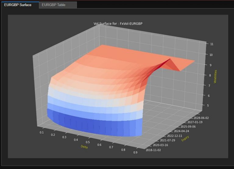
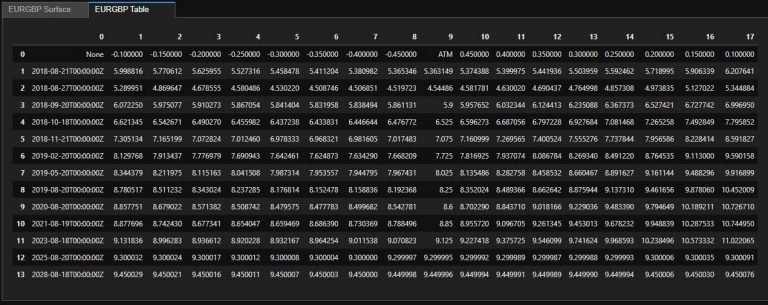
References
You can find more detail regarding the APIs and related technologies/articles for this notebook from the following resources:
- Refinitiv Eikon Data API page on the Refinitiv Developer Community web site.
- Refinitiv Data API.
- Instrument Pricing Analytics — Volatility Surfaces and Curves
- How to display matplotlib plots in a Jupyter tab widget?
- Shout out to Evgeny Kovalyov and his work on the Refinitiv Side by Side API
For any question related to this article or Refinitiv APIs, please use the Developers Community Q&A Forum.