Author:

Last Updated: Jan 2026
With tens of thousands of stocks to choose from, how do we go about selecting a few worth buying? Stock news, uncertainty and emotions add to the bitterness of this process. Whatever some experts suggest, it is impossible to go through all balance sheets to identify companies with low net debt and improving net profit margins.
This article uses a simple quantitative momentum strategy using Python and Refinitiv's DataScope Select (DSS) API to filter and select the best Intraday stocks. Given the breadth of the reference and pricing data available via DataScope Select, the APIs are ideal to build desktop applications which need a data source to populate data fields and graphs.
The DataScope Select APIs offer programmatic access to Refinitiv content in a more flexible way than the browser- and FTP-based data access solutions. They can be used to create an infinite number of client applications written in any desired programming language, for example, C#, C++, Visual Basic, Java, Objective-C and Swift. It supports the management of instrument and entity lists, report templates and schedules for the purpose of requesting extractions. It also supports higher level calls that can make data extractions directly, without requiring the creation of instrument lists, report templates or schedules on the DSS server.
Prerequisites
To run the example in this article we will need:
- Access to DataScope Select (DSS) API
- Python 3.7-3.9
- Required Python Packages: pandas, numpy, matplotlib, seaborn, scipy, requests
What is Quantitative Momentum Strategy?
In Physics, the term Momentum is used to define an object’s quantity and direction of motion. Similarly in financial markets, the momentum of an asset is the direction and speed of price change of the asset in the market. It is considered a primary stock factor (a.k.a anomaly, or smart-beta factor) affecting stock returns and has been outperforming the stock indices all over the world.
Quantitative Momentum is an investment strategy which selects stocks for investment whose price increased the most during a period. It is the process of identifying stocks with a great uptrend.
Let's see how this strategy can be implemented in Python using DSS API.
Importing required Packages
import os
import gzip
import pandas as pd
import requests
import numpy as np
from scipy.stats import percentileofscore as score
from math import floor
from json import dumps, loads
from requests import get, post
from time import sleep
from getpass import getpass, GetPassWarning
from collections import OrderedDict
import matplotlib
import matplotlib.pyplot as plt
import seaborn as sns
matplotlib.rc_file_defaults()
Here, Pandas package is used to deal with data, the NumPy package is used to work with arrays, the Requests package is used to pull data using DSS API, the Math package is used for mathematical functions, the SciPy package is used for complex functions, and few other packages are also used for support.
After importing all the required packages into our python environment, let's define a function to authenticate connection with DSS API.
def RequestNewToken(username="",password=""):
'''
username: DSS API login id
password: DSS API login password
'''
_AuthenURL = "https://selectapi.datascope.lseg.com/RestApi/v1/Authentication/RequestToken"
_header= {}
_header['Prefer']='respond-async'
_header['Content-Type']='application/json; odata.metadata=minimal'
_data={'Credentials':{
'Password':password,
'Username':username
}
}
print("Send Login request")
resp=post(_AuthenURL,json=_data,headers=_header)
if resp.status_code!=200:
message="Authentication Error Status Code: "+ str(resp.status_code) +" Message:"+dumps(loads(resp.text),indent=4)
raise Exception(str(message))
return loads(resp.text)['value']
At this step, we will take DSS username and password as input from user.
_DSSUsername = input('Username: ')
_DSSPassword = getpass('Password: ')
try:
# Requesting for authentication token which will be used further for fetching data
_token = RequestNewToken(_DSSUsername,_DSSPassword)
print("Token="+_token+"\n")
except GetPassWarning as e:
print(e)
def ExpandChain(token,json_payload):
'''
token: Authentication token generated from the above step
json_payload: Sample json object which application parses to get the RIC list by accessing the value of Constituents.
'''
_expandChainURL = "https://selectapi.datascope.lseg.com/RestApi/v1/Search/HistoricalChainResolution"
_header = {}
_header['Prefer'] = 'respond-async'
_header['Content-Type'] = 'application/json; odata.metadata=minimal'
_header['Accept-Charset'] = 'UTF-8'
_header['Authorization'] = 'Token' + token
resp = post(_expandChainURL, data=None, json=json_payload, headers=_header)
dataFrame= pd.DataFrame()
if(resp.status_code==200):
# Loads text from response as JSON object
json_object=loads(resp.text,object_pairs_hook=OrderedDict)
if len(json_object['value']) > 0:
# Parsing the JSON object and loading it to a dataframe
dataFrame = pd.DataFrame.from_dict(json_object['value'][0]['Constituents'])
else:
print("Unable to expand chain response return status code:",resp.status_code)
return dataFrame
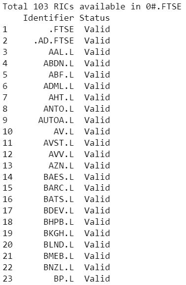
In the above code, we have used DSS API to extract the RICs and it's status of the stocks available in the FTSE 100 by sending request to DSS's RestAPI using request package. This function will post the request to HistoricalChainResolution and will return the data in dataframe format.
_chainRIC = "0#.FTSE"
_startDate = "2022-01-13"
_endDate = "2022-01-13"
try:
if(_token!=""):
# Sample JSON body for getting list of RICs in FTSE
_jsonquery={
"Request": {
"ChainRics": [
_chainRIC
],
"Range": {
"Start": _startDate,
"End": _endDate
}
}
}
# Calling ExpandChain function to get the list of RICs and it's status
df=ExpandChain(_token,_jsonquery)
if df.empty:
print("Unable to expand chain "+_chainRIC)
else:
ricCount=len(df['Identifier'])
print("Total "+str(ricCount)+" RICs available in "+ _chainRIC)
# Filter and print only RIC name and Status columns
pd.set_option('display.max_rows', ricCount)
ftse_ric = df.filter(items=['Identifier','Status'])
ftse_ric.index = np.arange(1,len(ftse_ric)+1)
print(ftse_ric)
pd.reset_option('display.max_rows')
except Exception as ex:
print("Exception occrus:", ex)
# List of RICs available in FTSE100
ftse_list = ftse_ric.Identifier.values
print(ftse_list)
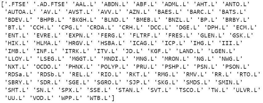
We first extracted the RICs and Status of the stocks in the FTSE 100 using the ExpandChain function and stored it into the ftse_ric dataframe. Then we defined a variable ‘ftse_list’ to store the extracted data into a NumPy array.
To learn more about "How to expand Chain RIC using the Tick History REST API in Python", visit here.
Pulling Intraday data of all the stocks in the FTSE using DataScope Select API
We have seen list of all the FTSE 100 stock’s RICs, now let’s pull some intraday data using DSS API.
For this let's define a function to extract data first for the given ChainRic, i.e., #0.FTSE.
def ExtractRaw(token,json_payload):
try:
_extractRawURL="https://selectapi.datascope.lseg.com/RestApi/v1/Extractions/ExtractRaw"
# Setup Request Header
_header={}
_header['Prefer']='respond-async'
_header['Content-Type']='application/json; odata.metadata=minimal'
_header['Accept-Charset']='UTF-8'
_header['Authorization']='Token'+token
# Post Http Request to DSS server using extract raw URL
resp=post(_extractRawURL,data=None,json=json_payload,headers=_header)
# Print Status Code return from HTTP Response
print("Status Code="+str(resp.status_code) )
# Raise exception with error message if the returned status is not 202 (Accepted) or 200 (Ok)
if resp.status_code!=200:
if resp.status_code!=202:
message="Error: Status Code:"+str(resp.status_code)+" Message:"+resp.text
raise Exception(message)
# Get location from header, URL must be https so we need to change it using string replace function
_location=str.replace(resp.headers['Location'],"http://","https://")
print("Get Status from "+str(_location))
_jobID=""
# Pooling loop to check request status every 30 sec.
while True:
resp=get(_location,headers=_header)
_pollstatus = int(resp.status_code)
if _pollstatus==200:
break
else:
print("Status:"+str(resp.headers['Status']))
sleep(retryInterval) # wait for _retyInterval period and re-request the status to check if it already completed
# Get the jobID from HTTP response
json_resp = loads(resp.text)
_jobID = json_resp.get('JobId')
print("Status is completed the JobID is "+ str(_jobID)+ "\n")
# Check if the response contains Notes.If the note exists print it to console.
if len(json_resp.get('Notes')) > 0:
print("Notes:\n======================================")
for var in json_resp.get('Notes'):
print(var)
print("======================================\n")
# Request should be completed then Get the result by passing jobID to RAWExtractionResults URL
_getResultURL = str("https://selectapi.datascope.lseg.com/RestApi/v1/Extractions/RawExtractionResults(\'" + _jobID + "\')/$value")
print("Retrieve result from " + _getResultURL)
resp=get(_getResultURL,headers=_header,stream=True)
# Write Output to file
outputfilepath = str("FTSE_100_" + str(os.getpid()) + '.csv.gz')
if resp.status_code==200:
with open(outputfilepath, 'wb') as f:
f.write(resp.raw.read())
# Read data from csv.gz and shows output from dataframe head() and tail()
df=pd.read_csv(outputfilepath,compression='gzip')
return df
except Exception as ex:
print("Exception occrus:", ex)
In the above function as well, we have used DSS API to extract the data for all the RICs of FTSE 100 by sending request to DSS's RestAPI using request package. We first setup the request header and post the request to ExtractRaw to fetch data.
The fetched data will be written to a csv file using gzip compression, which will be loaded to a dataframe and returned.
In case, if there will be any exception it will be raised, for example if the request's returned status is not Accepted or Ok.
# value in second used by Pooling loop to check request status on the server
retryInterval=int(30)
# Sample JSON for FTSE ChainRic for pulling data within the given date range
ftse_json = {
"ExtractionRequest": {
"@odata.type": "#DataScope.Select.Api.Extractions.ExtractionRequests.TickHistoryIntradaySummariesExtractionRequest",
"ContentFieldNames": [
"High",
"Last",
"Low",
"Open",
"Volume"
],
"IdentifierList": {
"@odata.type": "#DataScope.Select.Api.Extractions.ExtractionRequests.InstrumentIdentifierList",
"InstrumentIdentifiers": [{
"Identifier": "0#.FTSE",
"IdentifierType": "ChainRIC"
}
],
"UseUserPreferencesForValidationOptions" : "False"
},
"Condition": {
"MessageTimeStampIn": "LocalExchangeTime",
"ReportDateRangeType": "Range",
"QueryStartDate": "2022-01-13T00:00:00.000000000Z",
"QueryEndDate": "2022-01-13T23:59:59.999999999Z",
"SummaryInterval": "OneMinute",
"DisplaySourceRIC": "True"
}
}
}
Here, we have defined retryInterval variable for re-requesting the status after it's value (in second) to check if post request is already completed.
# Read the HTTP request body for the FTSE JSON defined above.
ftse_df = ExtractRaw(_token,ftse_json)
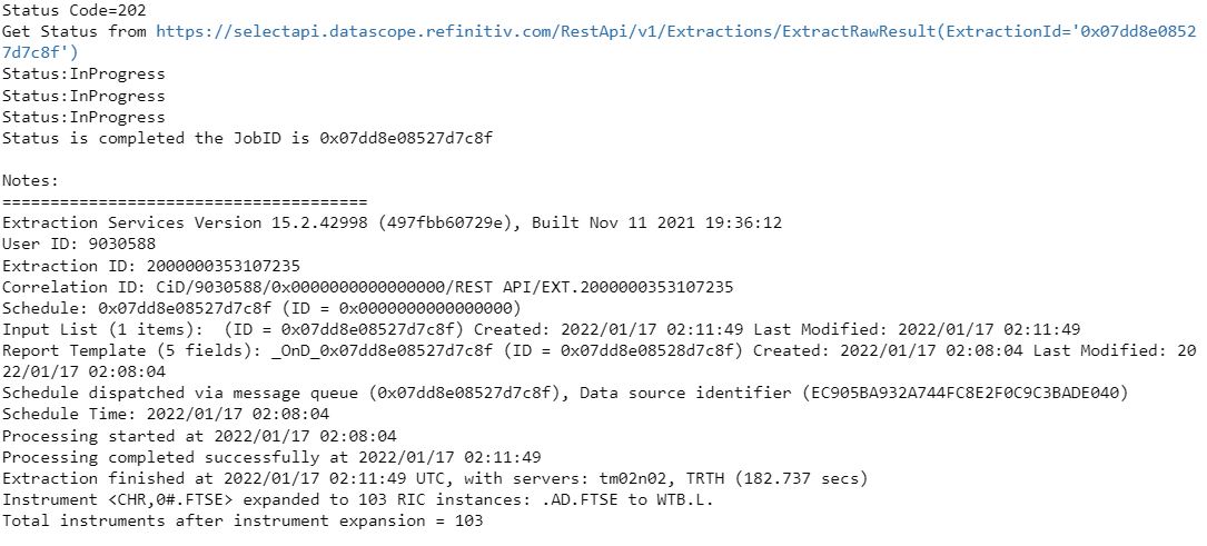
Here, we can see the Status and progress of the ExtractRaw function. Once the data is fetched completely, few metadata for each of the RICs is also displayed such as #RIC, Domain, Start, End, Status, and Count. We can also view all the data values fetched using the last url printed at the end.
ftse_df.head()
If you don’t know how to pull stock data using DSS API, I suggest to read article on it here.
Data Pre-Processing
At this step, we will pre-process the data to get it ready in the desired format.
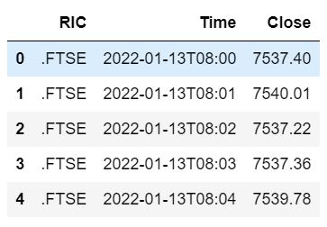
1. First format the date-time column and select the columns which we need further for our strategy.
# Formatting Date-Time column for just keeping date, hours and minutes in that column
ftse_df['Date-Time'] = ftse_df['Date-Time'].apply(lambda x: x.split('.')[0][:-3])
# Subsetting the dataframe only for columns required further for strategy and renaming them
ftse_df = ftse_df[['#RIC', 'Date-Time', 'Last']]
ftse_df.columns = ['RIC', 'Time', 'Close']
ftse_df.head()
2. Transpose the dataframe so that RICs name become the column names, set the date-time column as index, and Close values in there corresponding columns.
ftse_df_list = []
# Transforming all the RICs in column names and replacing the values with respective Closing prics of the Rics under them
for ric in ftse_list:
temp_df = ftse_df[ftse_df['RIC']==ric][['Time', 'Close']]
temp_df.columns = ['Time', ric]
temp_df = temp_df.set_index('Time')
ftse_df_list.append(temp_df)
final_ftse_df = pd.concat(ftse_df_list, axis=1)
# Sorting DataFrame and index based on date-time
final_ftse_df.sort_index(inplace=True)
# Dropping columns with all null values
final_ftse_df.dropna(how='all', axis=1, inplace=True)
final_ftse_df.head()
Since, now the data is ready in the desired format, now we will save the extracted intraday data of all FTSE 100 stocks. We also dropped column with all null values. It is an optional step but a good practice to save time, so first saving the extracted intraday data in the name of ‘ftse100’ using the ‘to_csv’ function provided by the Pandas package.
# Optional Step
final_ftse_df.to_csv('ftse100.csv')
Calculating Percentage Change and Momentum
Next we are the going to calculate change in percentage and momentum of all the stocks
# Calculating Percentage Change using pct_change function of pandas
dc = []
for i in final_ftse_df.columns:
dc.append(final_ftse_df[i].pct_change().sum())
ftse100_momentum = pd.DataFrame(columns = ['symbol', 'day_change'])
ftse100_momentum['symbol'] = final_ftse_df.columns
ftse100_momentum['day_change'] = dc
# Calculating Momentum
ftse100_momentum['momentum'] = 'N/A'
for i in range(len(ftse100_momentum)):
ftse100_momentum.loc[i, 'momentum'] = score(ftse100_momentum.day_change, ftse100_momentum.loc[i, 'day_change'])/100
ftse100_momentum['momentum'] = ftse100_momentum['momentum'].astype(float)
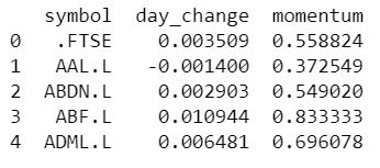
print(ftse100_momentum.head())
First, we created an empty list named dc to store the percentage change of each stock. Using for loop, we are iterating over the RICs of all the stocks in the FTSE 100 and appended the calculated percentage change using the ‘pct_change’ function provided by the Pandas package into the ‘dc’ list. Then we created a dataframe named ftse100_momentum to store the symbol of the stock, percentage change, and the momentum which we calculated after this.
To calculate the momentum, we first created a column named ‘momentum’ in the ‘ftse100_momentum’ dataframe and filled it with null values. Then we passed on a for-loop to fill the null values with the actual momentum values.
Finding Stocks with Greater Momentum
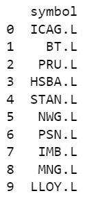
First, we will create a dataframe named ‘top_picks’ which stores the top 10 stocks having greater momentum than the rest.
In order to sort and find the top 10 stocks, we used the ‘nlargest’ function provided by the Pandas package.
top_picks = ftse100_momentum.nlargest(10, 'momentum')['symbol'].reset_index().drop('index', axis = 1)
print(top_picks)
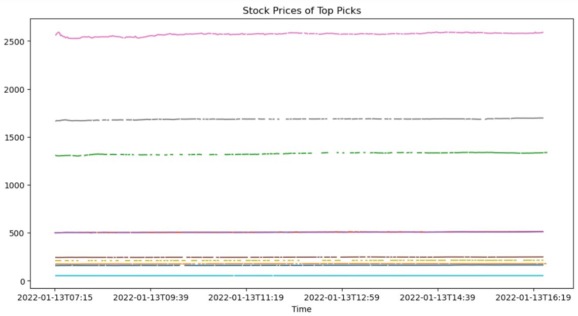
for ticks in top_picks['symbol']:
final_ftse_df[ticks].plot(label = ticks, figsize = (12,6))
plt.title('Stock Prices of Top Picks')
plt.show()
Backtesting the strategy
In this step, we are going to backtest Quantitative Momentum Strategy by investing money in the top 10 stocks with the highest momentum, and let’s see what results we get.
First, we will define two variables:
- One to store the total investment value
- And other to store the investment value per stock
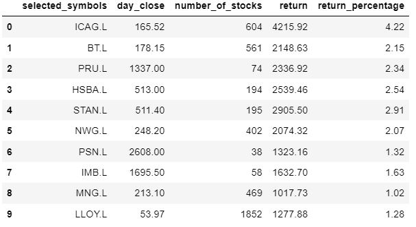
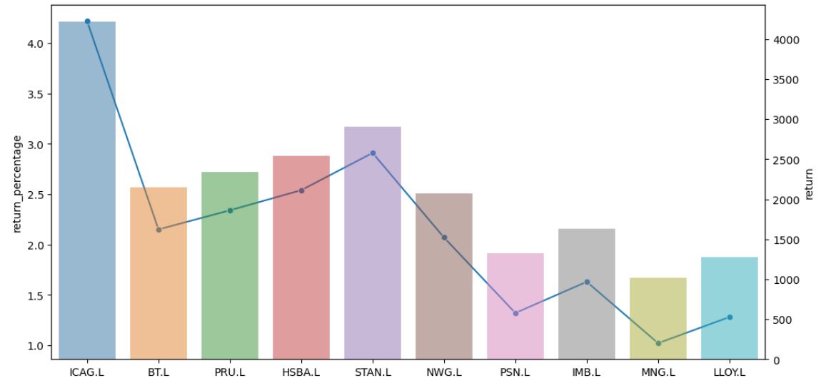
Next, we will use a for loop to find the day’s close price of all the top 10 stocks and append those values into the ‘day_close’ variable. In further lines of code, we will create a dataframe named ‘backtest_df’ which will be comprised of the calculated number of stocks to buy in each of them, the returns we got by investing in those top 10 stocks, and finally the return percentage of our investment.
# Backtesting the Strategy
# Creating a copy of ftse df
final_ftse_df_copy = final_ftse_df.copy()
final_ftse_df_copy.fillna(-1, inplace=True)
# Defining total value of portfolio to be invested for testing
portfolio_val = 1000000
# Calculating amount per select stocks which we got using momentum strategy
per_stock_val = portfolio_val/len(top_picks)
day_close = []
# filtering data for only those 10 stocks
for i in top_picks['symbol']:
data = final_ftse_df_copy[i]
j = -1
while data[j]==-1:
j -= 1
day_close.append(data[j])
backtest_df = pd.DataFrame(columns = ['selected_symbols', 'day_close', 'number_of_stocks', 'return', 'return_percentage'])
backtest_df['selected_symbols'] = top_picks['symbol']
backtest_df['day_close'] = day_close
for i in range(len(backtest_df)):
backtest_df.loc[i, 'number_of_stocks'] = floor(per_stock_val/day_close[i])
returns = []
for i in top_picks['symbol']:
ret = np.diff(final_ftse_df[i])
ret = ret[~np.isnan(ret)]
returns.append(round(sum(ret), 2))
backtest_returns = []
return_percentage = []
for i in range(len(backtest_df)):
br = returns[i]*backtest_df.loc[i, 'number_of_stocks']
rp = br/per_stock_val*100
backtest_returns.append(round(br, 2))
return_percentage.append(round(rp, 2))
backtest_df['return'] = backtest_returns
backtest_df['return_percentage'] = return_percentage
backtest_df
# Plotting return percantage on left scale of y-axis denoted by line chart and return values on right scale of y-axis denoted by bar chart
ax1 = sns.set_style(style=None, rc=None )
fig, ax1 = plt.subplots(figsize=(12,6))
sns.lineplot(data = backtest_df['return_percentage'], marker='o', sort = False, ax=ax1)
ax2 = ax1.twinx()
sns.barplot(data = backtest_df, x='selected_symbols', y='return', alpha=0.5, ax=ax2)
plt.show()
We have got some decent returns above!!
Conclusion
In this article, we learned about Quantitative Momentum Strategy and it's implementation in Python using DSS API to pick tradable stocks. We defined a function to authenticate with DSS Rest API and get a token, and further expanded FTSE ChainRic to get the list of all stocks of FTSE 100. We can consider stocks listed on other exchanges to experiment around as well. We defined another function to pull intraday data for FTSE ChainRic using DSS Rest API. By performing research given the amount of data being pulled, we can learn different ways of data extraction using DSS API along with extensive data processing. Further we can try tuning this strategy accordingly by using several other metrics.
Get In Touch
Source Code
Related APIs
Request Free Trial
Call your local sales team
Americas
All countries (toll free): +1 800 427 7570
Brazil: +55 11 47009629
Argentina: +54 11 53546700
Chile: +56 2 24838932
Mexico: +52 55 80005740
Colombia: +57 1 4419404
Europe, Middle East, Africa
Europe: +442045302020
Africa: +27 11 775 3188
Middle East & North Africa: 800035704182
Asia Pacific (Sub-Regional)
Australia & Pacific Islands: +612 8066 2494
China mainland: +86 10 6627 1095
Hong Kong & Macau: +852 3077 5499
India, Bangladesh, Nepal, Maldives & Sri Lanka:
+91 22 6180 7525
Indonesia: +622150960350
Japan: +813 6743 6515
Korea: +822 3478 4303
Malaysia & Brunei: +603 7 724 0502
New Zealand: +64 9913 6203
Philippines: 180 089 094 050 (Globe) or
180 014 410 639 (PLDT)
Singapore and all non-listed ASEAN Countries:
+65 6415 5484
Taiwan: +886 2 7734 4677
Thailand & Laos: +662 844 9576


