Market impact calculations

Dr. Marios Skevofylakas

Overview

In this article, we implement a theoretical system that aims to shed some light on one of the stochastic constituents of Transaction Cost Analysis (TCA) that of the market impact. We will start by presenting some of the theory behind TCA and then move on to the implementation and analysis of the market impact calculations.

With regards to the dataset, we will be using LSEG D&A libraries to ingest historical pricing data and use used to calculate the important components of market impact.

Theoretical background on TCA

Transaction Cost Analysis helps quantify the costs associated with executing investment trades. These costs can arise from a variety of sources and can significantly impact the profitability and efficiency of trade execution. The primary goal of TCA is to identify and measure these costs and enable traders to make better informed decisions that could lead to cost minimisation and improved execution performance.

TCA examines the deviation between the price at which trades are executed and the decision benchmark price. This difference is known as implementation shortfall and depicts the cost of materialising an investment idea in the actual markets. It is calculated as the difference of the returns of a paper traded portfolio, theoretically executed at decision prices and the actual executed portfolio.

There are several transaction cost constituents that sum up the final cost of a trade including fixed costs such as commissions and stochastic transaction costs such as spread. Market impact is a stochastic cost very much dependent on the view of the market landscape at the time of order execution.

Market Impact

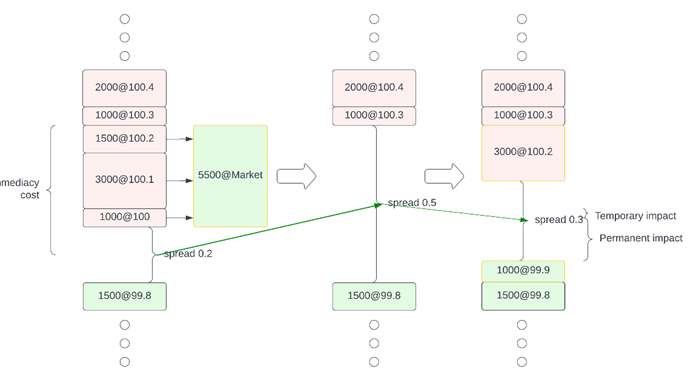
In this article we focus on market impact, defined as the difference between the price that would have prevailed if the trader’s own order was never executed in the market and the final execution price. Market impact is broken down into two components, temporary and permanent market impact. Temporary market impact is the sudden effect in price the trader’s liquidity demand has, and which will eventually be absorbed from the market. A high liquidity market can quickly absorb temporary market impact. The permanent market impact, however, is the long-term effect of the order execution has on the market. We could imagine for example a very aggressive market order traversing several layers of the orderbook and significantly affecting price temporarily. In the following theoretical graph such an order traverses three depth layers temporarily increasing the spread and mid-price and the market reacts by absorbing part of that impact.

Supply & Demand constituent

Let’s assume an initial stock price of initial_price GBP and that there is no drift or market memory. Let's also assume that buyers are always willing to cross the spread and the spread remains constant to bp_impact. All things remain equal, the markets should be able to absorb the supply and demand instantaneous shift. We assume an exponential decay of impact exponential_decay(x0, t, gamma=1) and we run the calculations for n ticks.

Import libraries and open the data session

Let's start by importing the necessary libraries and opening a data session.

    	
            import numpy as np
import matplotlib.pyplot as plt
import refinitiv.data as rd
 
from refinitiv.data.content import historical_pricing
from refinitiv.data.content.historical_pricing import Intervals
from refinitiv.data.content.historical_pricing import MarketSession
 
rd.open_session()

Get our data - one Line API call

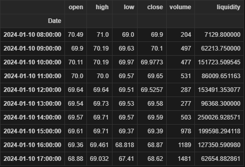
Here we use our get_data function to return hourly OHLCV for VOD.L for a single day’s worth of trading. Note the dataframe is already indexed on timestamp.

    	
            response = historical_pricing.summaries.Definition(
    universe = "VOD.L", 
    interval = Intervals.HOURLY,
    start='01-10-2024',
    end='01-11-2024',
    sessions = [
        MarketSession.NORMAL
    ],
    fields = ["OPEN_PRC", "HIGH_1", "LOW_1", "TRDPRC_1", "ACVOL_UNS"]
).get_data()
df = response.data.df
df.columns = ["open", "high", "low", "close", "volume"]

Calculating liquidity

For our market impact and impact absorption model we will need a surrogate of liquidity. This will allow as to calculate how fast the market landscape is able to respond to an order execution to mitigate its market impact. We calculate that by using the equation:

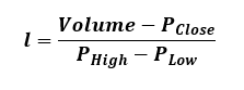
We then apply the calculation on our downloaded dataframe.

    	
            def liquidity_calc(x):
    return (x['volume'] * x['close']) / (x['high'] - x['low'])
 
df['liquidity'] = df.apply(liquidity_calc, axis=1)
df

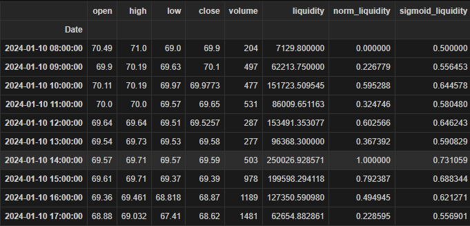
Next, we will need to apply a transformation function that will correctly scale liquidity so that it can be used from our theoretical model, we use the sigmoid function for that purpose and apply it to our dataset:

    	
            def sigmoid_liquidity(x):
    return 1/(1+np.exp(-x['norm_liquidity']))
 
df['sigmoid_liquidity'] = df.apply(sigmoid_liquidity, axis=1)
df

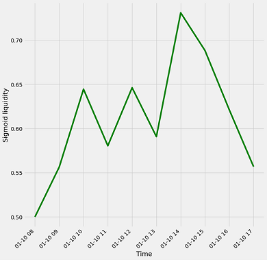
Let’s now plot sigmoid liquidity to examine its behaviour:

    	
            fig = plt.figure(figsize=(10,10))
plt.plot(df['sigmoid_liquidity'], color='green')
plt.xlabel("Time")
plt.ylabel("Sigmoid liquidity")
plt.xticks(rotation=45, ha="right")
plt.show()

We can now calculate the rate at which the market is able to absorb market impact for every one-hour period, using the following assumption of exponential decay:

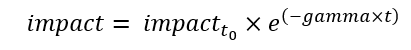
The following script applies hourly sigmoid liquidity and simulates absorption rates for a theoretical impact of 10bp.

    	
            bp_impact = 10
ticks = 20
initial_price = 1
 
def exponential_decay(x0, t, gamma=1):
    return x0 * np.exp(-gamma * t)
 
market = []
for ix, row in df.iterrows():
    mi = initial_price * bp_impact / 100 / 100
    mi_price = initial_price + mi
    market_hour = [mi_price] * ticks
    for t in range(1, ticks):
        market_hour[t] = initial_price + exponential_decay(mi, t, row['sigmoid_liquidity'])
    market.append(market_hour)

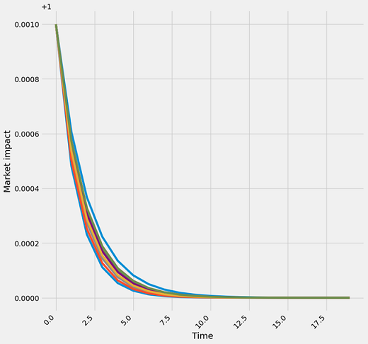
The following plot shows how quickly the market, depending on hourly liquidity, can absorb the 10bp impact. We can see the variation in behaviour with hours of low liquidity absorbing impact at a slower rate.

    	
            fig = plt.figure(figsize=(10,10))
for hour in market:
    plt.plot(hour)
plt.xlabel("Time")


plt.ylabel("Market impact")
plt.xticks(rotation=45, ha="right")
plt.show()

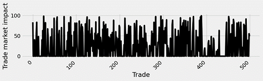
Let's now write a function that will simulate a scenario where multiple participants execute a trading schedule within a day with a probability of crossing the spread of trade_probability. We simulate a trading flow of n ticks and assume that each trade will cause an impact in the order book of min_bp to max_bp basis points.

    	
            min_bp = 10
max_bp = 100
 
ticks = 500
ticks_per_hour = int(ticks / len(df))
trade_probability = 0.45
 
def candle_trading_flow(ticks, trade_probability, min_bp, max_bp):
    trade_flow = (np.random.rand(ticks) > 1 - trade_probability).astype(int)
 
    impact_flow = []
    for trade in trade_flow:
        trade *= np.random.randint(min_bp, max_bp)
        impact_flow.append(trade)
       
    return trade_flow, impact_flow

Let’s first plot the trades and their impact within the day:

    	
            trade_flow, impact_flow = candle_trading_flow(ticks, trade_probability, min_bp, max_bp)
fig = plt.figure(figsize=(10,2))
plt.plot(impact_flow , color='black')
plt.xlabel("Trade")
plt.ylabel("Trade market impact")
plt.xticks(rotation=45, ha="right")
plt.show()

Next, we apply the theoretical model within each day to reveal impact results to price.

    	
            initial_price = 1
trade_flow_length = len(trade_flow)
market_price = [initial_price] * trade_flow_length
 
trade_impact = {}
 
hour_candle = 0 
for t in range(trade_flow_length):
    trade_impact[t] = []
    
for t1 in range(trade_flow_length):
    if ticks_per_hour % (t1+1) == 0:
        hour_candle += 1
    for t in range(t1):
        trade_impact[t1].append(0)
    for t2 in range(trade_flow_length - t1):
        if trade_flow[t1] == 1:
            mi = initial_price * impact_flow[t1] / 100 / 100
            market_price[t1 + t2] = (market_price[t1 + t2] + exponential_decay(mi, t2, df.iloc[hour_candle]['sigmoid_liquidity']))
            trade_impact[t1].append(exponential_decay(mi, t2, df.iloc[hour_candle]['sigmoid_liquidity']))

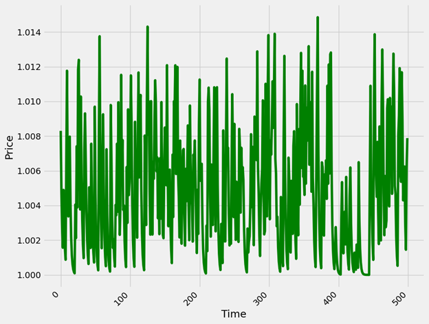
We can now see how this trading schedule affects the market price with hourly periods of higher liquidity being able to absorb trading flow impact resulting in price returning to its initial value. Another interesting phenomenon to observe is that around the 400th tick of the trading flow and as activity is lower it is much easier for the market to absorb market impact.

    	
            fig = plt.figure(figsize=(10,8))
plt.plot(market_price, color='green')
 
plt.xlabel("Time")
plt.ylabel("Price")
plt.xticks(rotation=45, ha="right")
plt.show()

Conclusions

In this article we explore a theoretical market impact absorption model to shed some light on market price dynamics. We ingest a day’s worth of hourly data using LSEG D&A data libraries and we calculate hourly liquidity. Using a sigmoid transformation, we bound liquidity and generate a gamma metric which we then use to calculate hourly market impact absorption rates. We can then simulate and observe market price dynamics during the day and better understand market impact and how trade flow aggressiveness can affect our own order's executions’ transaction costs.

If you would like to reach out with any questions regarding this article, we would be happy to address those in our Developer Community Q&A Forum.