

Generating Alpha using Starmine Analytical Models - a Python example
Overview
This article will demonstrate how we can use Starmine Analytical Models to derive insight and generate alpha, in this case, for equity markets. It is intended as a teaser to intice you to further explore this rich vein rather than a rigorous scientific study. I will be using LSEG Workspace and more specifically our LSEG Data Library for Python to access all the data I need to conduct this analysis - however Starmine Analytics is available in other products and delivery channels. I will also provide the Jupyter notebook source via gitub.
Pre-requisites:
LSEG Workspace with access to LSEG Data Library to Python (Free Trial Available)
Python 3.x
Required Python Packages: lseg-data, pandas, numpy, matplotlib, sklearn, scipy
Starmine Quantitative Analytics
In short - StarMine provides a suite of proprietary alpha-generating analytics and models spanning sectors, regions, and markets. The list of models is really broad-based and includes both quantitative analytics (such as smartEstimates) and quantitative models (such as the Combined Alpha Model I will demo here).
All of these analytics and models can provide you with new sources of information and subsequently alpha - they are calculated by our Starmine team and delivered to you - saving you many man years of work and research etc. You can find out more about Starmine Analytics by going here.
How to Access the Starmine and Other Data
As mentioned above I will be using LSEG Workspace and specifically our LSEG Data Library for Python - which is a really easy to use yet performant web API. At the time of writing this article it is still in Beta - but all LSEG Workspace users can access it and going to the developer portal here and follow instructions. If you have any questions around the API there are also monitored Q&A forums.
Once we have access to the LSEG Data Library for Python its very straightforward to get the data we need. First lets import some packages we will need to conduct this analysis and also set our App ID (this is available from the App ID generator - see the quick start guide for further details):
import lseg.data as ld
import pandas as pd
import numpy as np
import matplotlib.pyplot as plt
ld.open_session(app_key = '<APP KEY>')
Next we need to formulate our API call. In this case, I will be requesting data for all CAC-40 index constituents and I will be requesting a mixture of both Reference, Starmine Analytics and Price performance data for 8 quarters - I have made it more generic here - but essentially this is one line of code! And as you will see the API returns the data in a pandas dataframe.
RICS = ['0#.FCHI']
fields =['TR.TRBCIndustryGroup','TR.CombinedAlphaCountryRank(SDate=0,EDate=-7,Frq=FQ)','TR.CombinedAlphaCountryRank(SDate=0,EDate=-7,Frq=FQ).Date',
'TR.TotalReturn3Mo(SDate=0,EDate=-7,Frq=FQ)','TR.TotalReturn3Mo(SDate=0,EDate=-7,Frq=FQ).calcdate']
ids = ld.get_data(
universe = RICS,
fields = fields)
ids.head(20)
| Instrument | TRBC Industry Group Name | Combined Alpha Model Country Rank | Date | 3 Month Total Return | Calc Date | |
|---|---|---|---|---|---|---|
| 0 | MICP.PA | Automobiles & Auto Parts | 26 | 2025-06-30 | -0.495302 | 2025-06-30 |
| 1 | MICP.PA | 61 | 2025-03-31 | 1.918239 | 2025-03-31 | |
| 2 | MICP.PA | 62 | 2024-12-31 | -12.78113 | 2024-12-31 | |
| 3 | MICP.PA | 92 | 2024-09-30 | 0.969261 | 2024-09-30 | |
| 4 | MICP.PA | 96 | 2024-06-30 | 5.447033 | 2024-06-30 | |
| 5 | MICP.PA | 91 | 2024-03-31 | 9.426987 | 2024-03-31 | |
| 6 | MICP.PA | 84 | 2023-12-31 | 11.661507 | 2023-12-31 | |
| 7 | MICP.PA | 78 | 2023-09-30 | 7.427938 | 2023-09-30 | |
| 8 | LEGD.PA | Machinery, Tools, Heavy Vehicles, Trains & Ships | 43 | 2025-06-30 | 17.187581 | 2025-06-30 |
| 9 | LEGD.PA | 60 | 2025-03-31 | 3.402807 | 2025-03-31 | |
| 10 | LEGD.PA | 41 | 2024-12-31 | -8.964182 | 2024-12-31 | |
| 11 | LEGD.PA | 84 | 2024-09-30 | 11.506908 | 2024-09-30 | |
| 12 | LEGD.PA | 63 | 2024-06-30 | -3.691957 | 2024-06-30 | |
| 13 | LEGD.PA | 64 | 2024-03-31 | 4.378321 | 2024-03-31 | |
| 14 | LEGD.PA | 51 | 2023-12-31 | 7.789233 | 2023-12-31 | |
| 15 | LEGD.PA | 47 | 2023-09-30 | -3.854626 | 2023-09-30 | |
| 16 | BNPP.PA | Banking Services | 73 | 2025-06-30 | 3.193466 | 2025-06-30 |
| 17 | BNPP.PA | 91 | 2025-03-31 | 29.871665 | 2025-03-31 | |
| 18 | BNPP.PA | 61 | 2024-12-31 | -3.78554 | 2024-12-31 | |
| 19 | BNPP.PA | 50 | 2024-09-30 | 3.393247 | 2024-09-30 |
Now that we have our data in a dataframe we may need to do some wrangling to get the types correctly set. The get_data call is the most flexible of calls so this is to be expected. We can easily check the types of data in the dataframe by column:
ids.info()
<class 'pandas.core.frame.DataFrame'>
RangeIndex: 320 entries, 0 to 319
Data columns (total 6 columns):
# Column Non-Null Count Dtype
--- ------ -------------- -----
0 Instrument 320 non-null string
1 TRBC Industry Group Name 320 non-null string
2 Combined Alpha Model Country Rank 320 non-null Int64
3 Date 320 non-null datetime64[ns]
4 3 Month Total Return 320 non-null Float64
5 Calc Date 320 non-null datetime64[ns]
dtypes: Float64(1), Int64(1), datetime64[ns](2), string(2)
memory usage: 15.8 KB
First we want to cast the Date object (a string) as a datetime type, then we want to set that datetime field as the index for the frame. Secondly, we want to make sure any numeric fields are numeric and any text fields are strings:
ids['Date']=pd.to_datetime(ids['Date'])
ads=ids.set_index('Date')[['Instrument','TRBC Industry Group Name','Combined Alpha Model Country Rank','3 Month Total Return']]
ads['3 Month Total Return'] = pd.to_numeric(ads['3 Month Total Return'], errors='coerse')
ads['TRBC Industry Group Name'] = ads['TRBC Industry Group Name'].astype(str)
ads.head(10)
| Instrument | TRBC Industry Group Name | Combined Alpha Model Country Rank | 3 Month Total Return | |
|---|---|---|---|---|
| Date | ||||
| 2025-06-30 | MICP.PA | Automobiles & Auto Parts | 26 | -0.495302 |
| 2025-03-31 | MICP.PA | 61 | 1.918239 | |
| 2024-12-31 | MICP.PA | 62 | -12.78113 | |
| 2024-09-30 | MICP.PA | 92 | 0.969261 | |
| 2024-06-30 | MICP.PA | 96 | 5.447033 | |
| 2024-03-31 | MICP.PA | 91 | 9.426987 | |
| 2023-12-31 | MICP.PA | 84 | 11.661507 | |
| 2023-09-30 | MICP.PA | 78 | 7.427938 | |
| 2025-06-30 | LEGD.PA | Machinery, Tools, Heavy Vehicles, Trains & Ships | 43 | 17.187581 |
| 2025-03-31 | LEGD.PA | 60 | 3.402807 |
ads.dtypes
Instrument string[python]
TRBC Industry Group Name object
Combined Alpha Model Country Rank Int64
3 Month Total Return Float64
dtype: object
ads.head()
| Instrument | TRBC Industry Group Name | Combined Alpha Model Country Rank | 3 Month Total Return | |
|---|---|---|---|---|
| Date | ||||
| 2025-06-30 | MICP.PA | Automobiles & Auto Parts | 26 | -0.495302 |
| 2025-03-31 | MICP.PA | 61 | 1.918239 | |
| 2024-12-31 | MICP.PA | 62 | -12.78113 | |
| 2024-09-30 | MICP.PA | 92 | 0.969261 | |
| 2024-06-30 | MICP.PA | 96 | 5.447033 |
A bit more wrangling is required here as we can see for example that the API has returned the TRBC Industry Group only for the most current instance of each instrument - not for the historical quarters. We can recitfy this easily in 2 lines of code. First we will replace blanks with nan (not a number). We can then use the excellent and surgical fillna dataframe function to fill the Sector name to the historic quarters:
ads1 = ads.replace('', np.nan, regex=True)
ads1['TRBC Industry Group Name'].fillna(method='ffill',limit=7, inplace=True)
ads1.head(15)
| Instrument | TRBC Industry Group Name | Combined Alpha Model Country Rank | 3 Month Total Return | |
|---|---|---|---|---|
| Date | ||||
| 2025-06-30 | MICP.PA | Automobiles & Auto Parts | 26 | -0.495302 |
| 2025-03-31 | MICP.PA | NaN | 61 | 1.918239 |
| 2024-12-31 | MICP.PA | NaN | 62 | -12.78113 |
| 2024-09-30 | MICP.PA | NaN | 92 | 0.969261 |
| 2024-06-30 | MICP.PA | NaN | 96 | 5.447033 |
| 2024-03-31 | MICP.PA | NaN | 91 | 9.426987 |
| 2023-12-31 | MICP.PA | NaN | 84 | 11.661507 |
| 2023-09-30 | MICP.PA | NaN | 78 | 7.427938 |
| 2025-06-30 | LEGD.PA | Machinery, Tools, Heavy Vehicles, Trains & Ships | 43 | 17.187581 |
| 2025-03-31 | LEGD.PA | NaN | 60 | 3.402807 |
| 2024-12-31 | LEGD.PA | NaN | 41 | -8.964182 |
| 2024-09-30 | LEGD.PA | NaN | 84 | 11.506908 |
| 2024-06-30 | LEGD.PA | NaN | 63 | -3.691957 |
| 2024-03-31 | LEGD.PA | NaN | 64 | 4.378321 |
| 2023-12-31 | LEGD.PA | NaN | 51 | 7.789233 |
We now need to shift the 3 Month Total Return column down by 1 so we can map CAM ranks to forward looking performance. Thankfully in pandas this is trivial and note the Groupby instrument clause.
ads1['3 Month Total Return'] = ads1.groupby('Instrument')['3 Month Total Return'].shift()
ads1.head(15)
| Instrument | TRBC Industry Group Name | Combined Alpha Model Country Rank | 3 Month Total Return | |
|---|---|---|---|---|
| Date | ||||
| 2025-06-30 | MICP.PA | Automobiles & Auto Parts | 26 | -0.495302 |
| 2025-03-31 | MICP.PA | NaN | 61 | 1.918239 |
| 2024-12-31 | MICP.PA | NaN | 62 | -12.78113 |
| 2024-09-30 | MICP.PA | NaN | 92 | 0.969261 |
| 2024-06-30 | MICP.PA | NaN | 96 | 5.447033 |
| 2024-03-31 | MICP.PA | NaN | 91 | 9.426987 |
| 2023-12-31 | MICP.PA | NaN | 84 | 11.661507 |
| 2023-09-30 | MICP.PA | NaN | 78 | 7.427938 |
| 2025-06-30 | LEGD.PA | Machinery, Tools, Heavy Vehicles, Trains & Ships | 43 | 17.187581 |
| 2025-03-31 | LEGD.PA | NaN | 60 | 3.402807 |
| 2024-12-31 | LEGD.PA | NaN | 41 | -8.964182 |
| 2024-09-30 | LEGD.PA | NaN | 84 | 11.506908 |
| 2024-06-30 | LEGD.PA | NaN | 63 | -3.691957 |
| 2024-03-31 | LEGD.PA | NaN | 64 | 4.378321 |
| 2023-12-31 | LEGD.PA | NaN | 51 | 7.789233 |
ads1.info()
<class 'pandas.core.frame.DataFrame'>
DatetimeIndex: 40 entries, 2025-06-30 to 2025-06-30
Data columns (total 4 columns):
# Column Non-Null Count Dtype
--- ------ -------------- -----
0 Instrument 40 non-null string
1 TRBC Industry Group Name 40 non-null object
2 Combined Alpha Model Country Rank 40 non-null Int64
3 3 Month Total Return 40 non-null Float64
dtypes: Float64(1), Int64(1), object(1), string(1)
memory usage: 1.6+ KB
ads1.dropna(axis=0, how='any', inplace=True)
ads1.head(20)
| Instrument | TRBC Industry Group Name | Combined Alpha Model Country Rank | 3 Month Total Return | |
|---|---|---|---|---|
| Date | ||||
| 2025-06-30 | MICP.PA | Automobiles & Auto Parts | 26 | -0.495302 |
| 2025-06-30 | LEGD.PA | Machinery, Tools, Heavy Vehicles, Trains & Ships | 43 | 17.187581 |
| 2025-06-30 | BNPP.PA | Banking Services | 73 | 3.193466 |
| 2025-06-30 | MT.AS | Metals & Mining | 86 | 1.076553 |
| 2025-06-30 | PUBP.PA | Media & Publishing | 62 | 6.311111 |
| 2025-06-30 | BOUY.PA | Construction & Engineering | 89 | 9.548732 |
| 2025-06-30 | VIE.PA | Multiline Utilities | 40 | -1.570987 |
| 2025-06-30 | EDEN.PA | Professional & Commercial Services | 49 | -11.29329 |
| 2025-06-30 | PRTP.PA | Specialty Retailers | 2 | -5.264399 |
| 2025-06-30 | LVMH.PA | Textiles & Apparel | 4 | -23.13524 |
| 2025-06-30 | AXAF.PA | Insurance | 96 | 9.647981 |
| 2025-06-30 | CAGR.PA | Banking Services | 66 | 1.196887 |
| 2025-06-30 | SOGN.PA | Banking Services | 93 | 16.679662 |
| 2025-06-30 | SCHN.PA | Machinery, Tools, Heavy Vehicles, Trains & Ships | 17 | 5.835198 |
| 2025-06-30 | SASY.PA | Pharmaceuticals | 42 | -17.073584 |
| 2025-06-30 | RENA.PA | Automobiles & Auto Parts | 38 | -13.736086 |
| 2025-06-30 | ENGIE.PA | Multiline Utilities | 95 | 19.697334 |
| 2025-06-30 | TEPRF.PA | Professional & Commercial Services | 49 | -10.541187 |
| 2025-06-30 | SAF.PA | Aerospace & Defense | 69 | 13.547759 |
| 2025-06-30 | ACCP.PA | Hotels & Entertainment Services | 31 | 6.471022 |
So now our Dataframe is seemingly in good shape - what are we going to do next? We can start with the question do higher CAM score leads to better performance? Or put more generically, are CAM scores RELATED to performance? Remember these CAM scores are dynamic and change overtime depending on changes in their underlying components AND relative to other companies in the universe (in this case companies in the same country).
So lets just see what this looks like in terms of a scatterplot for one sector of the CAC-40. Here we are just filtering the frame using a text filter and aggregating using a groupby statement. In this case we have 2 companies.
%matplotlib inline
adsl = ads1[ads1['TRBC Industry Group Name'] =='Professional & Commercial Services']
adsl = adsl.groupby('Instrument')
ax = adsl.plot(x='Combined Alpha Model Country Rank', y='3 Month Total Return', kind='scatter')
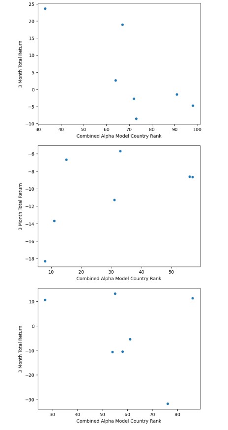
So lets be clear about what we are looking at. Each dot represents a pair of observations for CAM rank and 3M total return for a quarter - we should have 7 quarters of observations for each instrument. So we could implement a simple linear regression and that would have different parameters such as intercept, slope.
As I am in exploratory mode - I just am interested in the slope of the best fit linear line (of the form y = ax + b), where a is the slope coefficient. This should offer me some indication of how 3 Month total returns change for an increase in CAM rank. So our slope coefficient can tell us for example whether our variables are positively related (positive a) or negatively related (negative a) or really not related at all (near zero a).
We can also more formally calculate Spearman's Rank Correlation Coefficient which will give us a more rigorous measure of relatedness and also a probability that the null hypothesis (the two variables are not related) is true.
So rather than create plots for everything we can just create a model to provide the linear best fit solution for each instrument and then store that value in a new column as well as calculating the Spearman's Rank Correlation Coefficient and p-value.
First, I want to check for if any data is null as this may result in errors downstream.
ads1.isnull().any().count()
4
Here we can see there are 4 null values in our dataset - we can deal with these by replacing them with either mean values or most recent values. In our case, I choose the latter and will use a forward fill function to replace nulls:
adsNN = ads1.fillna(method='ffill')
adsNN.isnull().any()
Instrument False
TRBC Industry Group Name False
Combined Alpha Model Country Rank False
3 Month Total Return False
dtype: bool
Now we have confirmed we have no null values we can move on. Next we will use the Linear Regression model from the Linear Model tools from Scikit Learn package. We want to solve for 7 quarters of data for each Instrument. So we iterate over each intrument then use the model.fit method to generate the best fit linear solution (OLS) and then store the 'coef_' parameter of the model as a new column in the adsNN dataframe called 'slope'.
Whilst we are here we will also calculate a Spearman's Rank Correlation Coefficient using a routine from scipy package. The routine returns 2 values, the first is the Coefficient (Rho) and the second is the p-value. I just store these 2 elements in 2 seperate columns.
import sklearn
import scipy
from sklearn import linear_model
model = linear_model.LinearRegression()
for (group, adsNN_gp) in adsNN.groupby('Instrument'):
X=adsNN_gp[['Combined Alpha Model Country Rank']]
y=adsNN_gp[['3 Month Total Return']]
model.fit(X,y)
spearmans = scipy.stats.spearmanr(X,y)
adsNN.loc[adsNN.Instrument == adsNN_gp.iloc[0].Instrument, 'slope'] = model.coef_
adsNN.loc[adsNN.Instrument == adsNN_gp.iloc[0].Instrument, 'Rho'] = spearmans[0]
adsNN.loc[adsNN.Instrument == adsNN_gp.iloc[0].Instrument, 'p'] = spearmans[1]
adsNN.head(15)
| Instrument | TRBC Industry Group Name | Combined Alpha Model Country Rank | 3 Month Total Return | slope | Rho | p | |
|---|---|---|---|---|---|---|---|
| Date | |||||||
| 2025-03-31 | MICP.PA | Automobiles & Auto Parts | 61 | -0.495302 | -0.080008 | -0.178571 | 0.701658 |
| 2024-12-31 | MICP.PA | Automobiles & Auto Parts | 62 | 1.918239 | -0.080008 | -0.178571 | 0.701658 |
| 2024-09-30 | MICP.PA | Automobiles & Auto Parts | 92 | -12.78113 | -0.080008 | -0.178571 | 0.701658 |
| 2024-06-30 | MICP.PA | Automobiles & Auto Parts | 96 | 0.969261 | -0.080008 | -0.178571 | 0.701658 |
| 2024-03-31 | MICP.PA | Automobiles & Auto Parts | 91 | 5.447033 | -0.080008 | -0.178571 | 0.701658 |
| 2023-12-31 | MICP.PA | Automobiles & Auto Parts | 84 | 9.426987 | -0.080008 | -0.178571 | 0.701658 |
| 2023-09-30 | MICP.PA | Automobiles & Auto Parts | 78 | 11.661507 | -0.080008 | -0.178571 | 0.701658 |
| 2025-03-31 | LEGD.PA | Machinery, Tools, Heavy Vehicles, Trains & Ships | 60 | 17.187581 | -0.296857 | -0.357143 | 0.431611 |
| 2024-12-31 | LEGD.PA | Machinery, Tools, Heavy Vehicles, Trains & Ships | 41 | 3.402807 | -0.296857 | -0.357143 | 0.431611 |
| 2024-09-30 | LEGD.PA | Machinery, Tools, Heavy Vehicles, Trains & Ships | 84 | -8.964182 | -0.296857 | -0.357143 | 0.431611 |
| 2024-06-30 | LEGD.PA | Machinery, Tools, Heavy Vehicles, Trains & Ships | 63 | 11.506908 | -0.296857 | -0.357143 | 0.431611 |
| 2024-03-31 | LEGD.PA | Machinery, Tools, Heavy Vehicles, Trains & Ships | 64 | -3.691957 | -0.296857 | -0.357143 | 0.431611 |
| 2023-12-31 | LEGD.PA | Machinery, Tools, Heavy Vehicles, Trains & Ships | 51 | 4.378321 | -0.296857 | -0.357143 | 0.431611 |
| 2023-09-30 | LEGD.PA | Machinery, Tools, Heavy Vehicles, Trains & Ships | 47 | 7.789233 | -0.296857 | -0.357143 | 0.431611 |
| 2025-03-31 | BNPP.PA | Banking Services | 91 | 3.193466 | 0.094600 | 0.000000 | 1.000000 |
Voila - I have all the calculations I requested and I think I just want to average these by Instrument so I can get a summary view. (note averaging the slope, Rho and p values does not change them as they were calculated once for the 7 periods and just copied 7 times).
Averages = adsNN.groupby(['Instrument'])[["Combined Alpha Model Country Rank","3 Month Total Return", "slope","Rho","p"]].mean()
Averages
| Combined Alpha Model Country Rank | 3 Month Total Return | slope | Rho | p | |
|---|---|---|---|---|---|
| Instrument | |||||
| ACCP.PA | 69.0 | 6.078539 | 0.023852 | 0.126131 | 0.787572 |
| AIR.PA | 32.428571 | 6.158615 | -0.193148 | -0.071429 | 0.879048 |
| AIRP.PA | 50.428571 | 3.424774 | -0.141107 | -0.321429 | 0.482072 |
| AXAF.PA | 77.285714 | 7.523937 | 0.145741 | 0.180187 | 0.699046 |
| BNPP.PA | 57.285714 | 5.420644 | 0.094600 | 0.000000 | 1.000000 |
| BOUY.PA | 75.285714 | 4.252903 | -0.214687 | -0.142857 | 0.759945 |
| BVI.PA | 71.142857 | 3.954485 | -0.444660 | -0.785714 | 0.036238 |
| CAGR.PA | 77.714286 | 6.883497 | -0.227048 | -0.018019 | 0.969415 |
| CAPP.PA | 52.857143 | -1.321159 | 0.226137 | -0.126131 | 0.787572 |
| CARR.PA | 51.571429 | -2.054091 | -0.164072 | -0.214286 | 0.644512 |
| DANO.PA | 60.142857 | 5.254705 | 0.022856 | -0.254588 | 0.581668 |
| DAST.PA | 43.571429 | -1.502576 | -0.439090 | -0.792825 | 0.033444 |
| EDEN.PA | 30.142857 | -10.422603 | 0.114981 | 0.571429 | 0.180202 |
| ENGIE.PA | 85.0 | 7.664911 | -0.129615 | -0.018019 | 0.969415 |
| ESLX.PA | 60.714286 | 5.884667 | 0.400732 | 0.540562 | 0.210289 |
| EUFI.PA | 56.0 | 3.105955 | -0.577245 | -0.392857 | 0.383317 |
| HRMS.PA | 37.0 | 4.756075 | -0.359128 | -0.576600 | 0.175382 |
| LEGD.PA | 58.571429 | 4.51553 | -0.296857 | -0.357143 | 0.431611 |
| LVMH.PA | 9.0 | -5.757581 | 0.724143 | 0.345512 | 0.447816 |
| MICP.PA | 80.571429 | 2.306656 | -0.080008 | -0.178571 | 0.701658 |
| MT.AS | 48.142857 | 2.632894 | -0.320669 | -0.630656 | 0.128888 |
| ORAN.PA | 72.428571 | 5.189623 | -0.066211 | -0.142857 | 0.759945 |
| OREP.PA | 36.571429 | -0.383194 | 0.124258 | -0.035714 | 0.939408 |
| PERP.PA | 8.428571 | -7.72097 | 0.436047 | 0.054056 | 0.908365 |
| PRTP.PA | 4.571429 | -10.758458 | -0.400458 | -0.630488 | 0.129021 |
| PUBP.PA | 83.714286 | 4.768877 | -0.890684 | -0.846881 | 0.016197 |
| RENA.PA | 52.857143 | 2.181343 | -0.036580 | -0.250000 | 0.588724 |
| SAF.PA | 74.857143 | 9.857732 | -0.192011 | -0.392857 | 0.383317 |
| SASY.PA | 68.714286 | -1.451847 | -0.044428 | -0.250000 | 0.588724 |
| SCHN.PA | 57.285714 | 5.763114 | 0.145999 | 0.214286 | 0.644512 |
| SGEF.PA | 78.0 | 3.875607 | -0.110474 | -0.090094 | 0.847672 |
| SGOB.PA | 81.571429 | 8.384135 | 0.248954 | 0.535714 | 0.215217 |
| SOGN.PA | 46.857143 | 13.053266 | 0.515799 | 0.892857 | 0.006807 |
| STLAM.PA | 56.285714 | -6.564131 | 0.146212 | 0.072075 | 0.877959 |
| STMPA.PA | 27.285714 | -5.013044 | 0.077019 | -0.054056 | 0.908365 |
| TCFP.PA | 66.571429 | 12.566059 | -0.947059 | -0.486506 | 0.268249 |
| TEPRF.PA | 59.571429 | -3.331936 | -0.269440 | -0.071429 | 0.879048 |
| TTEF.PA | 58.857143 | -0.802727 | -0.083483 | -0.035714 | 0.939408 |
| URW.PA | 81.428571 | 10.268455 | -0.317900 | -0.270281 | 0.557731 |
| VIE.PA | 63.142857 | 2.763187 | 0.039597 | 0.109109 | 0.815871 |
Conclusion
So now we have a summarised view of our study - can we answer the question posited earlier? 'Are CAM scores RELATED to performance?' Let us have a look at average CAM score versus average 3 month total return (over 7 quarters). This seems to indicate that there is a slight positive relation between the two variables.
ax = Averages.plot(x='Combined Alpha Model Country Rank', y='3 Month Total Return', kind='scatter')
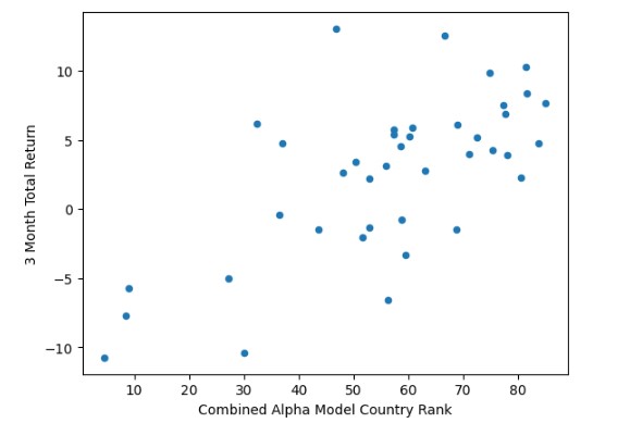
We can check this further by running the same Spearman's Rank Correlation Coefficient test against these summary results. Here we can see Rho of 50 which is both large & positive and with p of 0.101 the null hypothesis can be safetly rejected.
spearmans = scipy.stats.spearmanr(Averages['Combined Alpha Model Country Rank'],Averages['3 Month Total Return'])
Rho = spearmans[0]
p = spearmans[1]
print(Rho,p)
0.5891734710233015 6.341418985471288e-05
Further Resources for LSEG Data Library for Python
For Content Navigation in LSEG Workspace- please use the Data Item Browser Application: Type 'DIB' into Workspace Search Bar.