Last Updated: 28 Apr 2025
Modern Portfolio Theory
Economist Harry Markowitz introduced Modern Portfolio Theory in a 1952 publication in the Journal of Finance titled “Portfolio Selection”, which later earned him a Nobel Prize in Economics. Modern portfolio theory, or MPT (also known as mean-variance analysis), is a mathematical framework for assembling a portfolio of assets to maximize expected return for a given level of market risk. MPT argues that an investment's risk and return characteristics should not be viewed alone but should be evaluated by how the investment affects the overall portfolio's risk and return. MPT shows that an investor can construct a portfolio of multiple assets that will maximize returns for a given level of risk. Likewise, given a desired level of expected return, an investor can construct a portfolio with the lowest possible risk. Based on statistical measures such as variance and correlation, an individual investment's return is less important than how the investment behaves in the context of the entire portfolio. MPT assumes that investors are risk averse, meaning that given two portfolios that offer the same expected return, investors will prefer the one with less market risk. Conversely, an investor who wants higher expected returns must accept higher risk. The exact trade-off will not be the same for all investors. Different investors will evaluate the trade-off differently based on individual risk aversion characteristics. The implication is that a rational investor will not invest in a portfolio if a second portfolio exists with a more favorable risk-expected return profile – i.e., if for that level of risk an alternative portfolio exists that has better expected returns.
The expected return of the portfolio is calculated as a weighted sum of the individual assets' returns. The portfolio's risk is a function of the variances of each asset and the correlations of each pair of assets. To calculate the risk of a four-asset portfolio, an investor needs each of the four assets' variances and six correlation values, since there are six possible two-asset combinations with four assets. Because of the asset correlations, the total portfolio risk, or standard deviation, is lower than what would be calculated by a weighted sum.
Portfolio Optimization
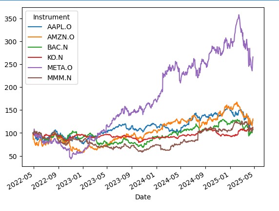
In our example we consider a portfolio of 6 large cap US stocks and we will optimize the portfolio, i.e. calculate the amount of each stock we need to hold in our portfolio to maximize the expected return for a given level of market risk (standard deviation of portfolio returns).
First we retrieve the daily price history for each stock for the last 3 years.
In [2]:
stocks_list = ['KO.N','AAPL.O','AMZN.O','META.O','BAC.N','MMM.N']
def get_prices(stocks, start_date):
stock_prices = ld.get_data(stocks,
['TR.PriceClose.date','TR.PriceClose'],
{'SDate':start_date, 'EDate':'0D'})
stock_prices['Price Close'] = stock_prices['Price Close'].astype('float64')
stock_prices['Date'] = pd.to_datetime(stock_prices['Date'])
stock_prices = stock_prices.set_index(['Date','Instrument'])
stock_prices = stock_prices.unstack()
stock_prices.columns = stock_prices.columns.get_level_values(1)
return stock_prices
prices = get_prices(stocks_list, start_date='-3Y')
ax = prices.rebase().plot()
Out [2]:
Then using f.fn library we calculate a bunch of stats for each stock including Sharpe and Sortino ratios.
In [3]:
np.seterr(all='ignore')
stats = prices.calc_stats()
stats.display()
Out [3]:
Stat AAPL.O AMZN.O BAC.N KO.N META.O MMM.N
------------------- ---------- ---------- ---------- ---------- ---------- ----------
Start 2022-04-28 2022-04-28 2022-04-28 2022-04-28 2022-04-28 2022-04-28
End 2025-04-25 2025-04-25 2025-04-25 2025-04-25 2025-04-25 2025-04-25
Risk-free rate 0.00% 0.00% 0.00% 0.00% 0.00% 0.00%
Total Return 27.89% 30.70% 7.82% 8.64% 166.01% 11.62%
Daily Sharpe 0.43 0.43 0.23 0.25 0.95 0.27
Daily Sortino 0.71 0.71 0.39 0.41 1.61 0.49
CAGR 8.57% 9.36% 2.55% 2.81% 38.67% 3.74%
Max Drawdown -33.43% -43.49% -34.83% -20.86% -60.20% -44.50%
Calmar Ratio 0.26 0.22 0.07 0.13 0.64 0.08
MTD -5.78% -0.67% -4.89% 0.40% -5.05% -6.50%
3m -6.06% -19.53% -14.68% 16.13% -15.48% -8.10%
6m -9.56% 0.62% -5.25% 7.46% -4.53% 10.08%
YTD -16.43% -13.86% -9.69% 15.50% -6.53% 6.38%
1Y 23.19% 8.82% 4.70% 16.47% 23.99% 50.22%
3Y (ann.) 8.57% 9.36% 2.55% 2.81% 38.67% 3.74%
5Y (ann.) - - - - - -
10Y (ann.) - - - - - -
Since Incep. (ann.) 8.57% 9.36% 2.55% 2.81% 38.67% 3.74%
Daily Sharpe 0.43 0.43 0.23 0.25 0.95 0.27
Daily Sortino 0.71 0.71 0.39 0.41 1.61 0.49
Daily Mean (ann.) 12.59% 16.10% 6.52% 4.10% 43.20% 8.48%
Daily Vol (ann.) 29.48% 37.69% 28.25% 16.20% 45.47% 31.29%
Daily Skew 0.52 -0.04 0.02 -0.45 0.44 2.01
Daily Kurt 8.25 4.33 4.11 4.69 17.39 27.88
Best Day 15.33% 12.18% 8.43% 4.73% 23.28% 22.99%
Worst Day -9.25% -14.05% -11.06% -6.96% -24.56% -11.03%
Monthly Sharpe 0.49 0.58 0.26 0.30 0.99 0.29
Monthly Sortino 1.01 1.28 0.47 0.52 1.85 0.59
Monthly Mean (ann.) 12.78% 19.19% 7.91% 4.77% 43.44% 9.51%
Monthly Vol (ann.) 26.29% 33.19% 29.91% 15.72% 43.79% 33.01%
Monthly Skew 0.29 0.61 -0.03 0.04 -0.40 0.42
Monthly Kurt -0.51 0.28 -0.27 0.77 0.56 -0.22
Best Month 18.86% 27.06% 19.34% 12.18% 26.77% 24.82%
Worst Month -12.23% -12.99% -16.62% -9.22% -31.34% -13.69%
Yearly Sharpe 0.62 0.78 0.36 0.40 0.83 0.50
Yearly Sortino 2.17 4.64 1.34 1.08 22.37 2.53
Yearly Mean 20.61% 37.14% 7.50% 4.60% 84.34% 12.92%
Yearly Vol 33.33% 47.78% 20.74% 11.46% 101.66% 25.67%
Yearly Skew -1.17 -0.67 1.17 -0.41 0.81 1.07
Yearly Kurt - - - - - -
Best Year 48.18% 80.88% 30.53% 15.50% 194.13% 41.24%
Worst Year -16.43% -13.86% -9.69% -7.36% -6.53% -8.84%
Avg. Drawdown -6.12% -6.66% -7.05% -6.34% -5.72% -8.00%
Avg. Drawdown Days 38.77 31.59 75.57 133.50 23.46 96.45
Avg. Up Month 6.91% 7.93% 7.10% 3.09% 10.78% 8.03%
Avg. Down Month -5.47% -7.26% -6.54% -3.84% -9.04% -7.30%
Win Year % 66.67% 66.67% 66.67% 66.67% 66.67% 66.67%
Win 12m % 92.31% 88.46% 53.85% 61.54% 100.00% 50.00%
Now let’s consider an initial portfolio with randomly assigned weights for each stock and calculate expected return and volatility of this portfolio.
In [4]:
# portfolio weights
weights = np.asarray([0.4,0.2,0.1,0.1,0.1,0.1])
returns = prices.pct_change()
# mean daily return and covariance of daily returns
mean_daily_returns = returns.mean()
cov_matrix = returns.cov()
# portfolio return and volatility
pf_return = round(np.sum(mean_daily_returns * weights) * 252, 3)
pf_std_dev = round(np.sqrt(np.dot(weights.T, np.dot(cov_matrix, weights))) * np.sqrt(252), 3)
print("Expected annualized return: " + "{:.1%}".format(pf_return))
print("Volatility: " + "{:.1%}".format(pf_std_dev))
Out [4]:
Expected annualized return: 14.5%
Volatility: 23.9%
Let's calculate portfolio weights that maximize Sharpe ratio and compare the return and volatility of this portfolio to our initial portfolio using pypfopt library.
In [5]:
# Expected returns and sample covariance
exp_returns = expected_returns.mean_historical_return(prices)
covar = risk_models.sample_cov(prices)
# Optimise portfolio for maximum Sharpe Ratio
ef = EfficientFrontier(exp_returns, covar)
raw_weights = ef.max_sharpe()
pf = ef.clean_weights()
print(pf)
perf = ef.portfolio_performance(verbose=True)
Out [5]:
OrderedDict({'AAPL.O': 0.0, 'AMZN.O': 0.0, 'BAC.N': 0.0, 'KO.N': 0.22332, 'META.O': 0.77668, 'MMM.N': 0.0})
Expected annual return: 30.9%
Annual volatility: 35.9%
Sharpe Ratio: 0.86
You see that in the previous step two stocks were removed from our portfolio (they were assigned zero weights). What if we allow short positions in our portfolio and optimize it by minimizing risk for a given target return?
In [6]:
ef = EfficientFrontier(exp_returns, covar, weight_bounds=(-1, 1))
pf = ef.efficient_return(target_return=perf[0])
print(pf)
perf = ef.portfolio_performance(verbose=True)
Out [6]:
OrderedDict({'AAPL.O': -0.0799275565306823, 'AMZN.O': -0.3474763064803908, 'BAC.N': -0.0848456313925584, 'KO.N': 0.710981114180169, 'META.O': 0.8536870274666907, 'MMM.N': -0.0524186472432282})
Expected annual return: 30.9%
Annual volatility: 32.8%
Sharpe Ratio: 0.94
Comparing the result with our long only portfolio for the same return we see slightly lower risk and higher Sharpe ratio.
The weights calculated for our optimized portfolio don't tell us how much of each stock we should hold. They may also result in fractional numbers of stocks, which is impractical. In the next step we use integer programming method to create discrete allocations for our portfolio. In other words given the cash amount we have to invest we calculate integer number for each stock holding and the amount of leftover cash.
In [7]:
latest_prices = discrete_allocation.get_latest_prices(prices)
allocation, leftover = discrete_allocation.DiscreteAllocation(pf, latest_prices,
total_portfolio_value=100000).lp_portfolio()
print(allocation)
print("Funds remaining: ${:.2f}".format(leftover))
Out [7]:
{'KO.N': 629, 'META.O': 100, 'AAPL.O': -38, 'AMZN.O': -184, 'BAC.N': -214, 'MMM.N': -38}
Funds remaining: $69.80
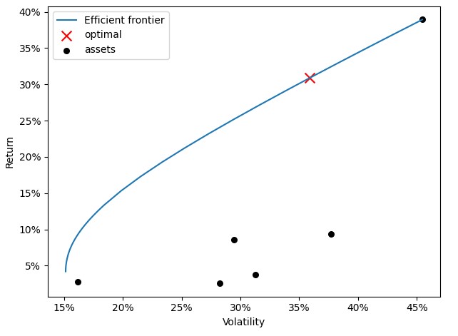
Efficient frontier
In modern portfolio theory, the efficient frontier is an investment portfolio which occupies the 'efficient' parts of the risk-return spectrum. Formally, it is the set of portfolios which satisfy the condition that no other portfolio exists with a higher expected return but with the same standard deviation of return. Using pypfopt library we calculate volatility and expected return on our portfolio given a range of target returns. When we plot calculated return against volatility we get classic textbook chart of efficient frontier for a portfolio without a risk free asset.
In [8]:
cla = CLA(exp_returns, covar)
ax = pypfopt.plotting.plot_efficient_frontier(cla, showfig = False)
ax.xaxis.set_major_formatter(FuncFormatter(lambda x, _: '{:.0%}'.format(x)))
ax.yaxis.set_major_formatter(FuncFormatter(lambda y, _: '{:.0%}'.format(y)))r(FuncFormatter(lambda y, _: '{:.0%}'.format(y)))
Out [8]:
Complete source code for this article can be downloaded from Github
https://github.com/LSEG-API-Samples/Article.LD.Python.PortfolioOptimization


