Discover our Data Library (part 2)

May 28,2025

Umer Nalla

Wasin Waeosri

Introduction to Data Library

This is Part 2 of this exploration of the new Library, so if you have not already done so - I recommend you check out Part 1 first.

The Data Library is latest evolution of library that provides a set of ease-of-use interfaces offering coders uniform access to the breadth and depth of financial data and services available on the Workspace, Delivery Platform, and Real-Time Platforms. You can find more details about the previous versions of libraries on Essential Guide to the Data Libraries - Generations of Python library (EDAPI, RDP, RD, LD) article.

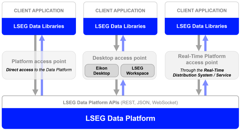
The library is available the following programming languages

This article is focusing on the Data Library for Python version 2 (LSEG Data Library, aka LD Library - As of May 2025).

One Library - Four Abstraction Layers

Just to recap, to cater to all developer types, the library offers 4 abstraction layers from the easiest to the slightly(!) more complex.

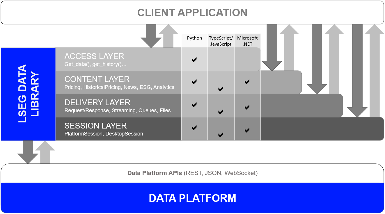
he four layers are as follows:

Access: Highest level - single function call to get data
Content: High level - Fuller response and logical market data objects
Delivery: Low level - lets developers interact with the platforms via various delivery modes (HTTP Request-Response, Stream, Queue, File)
Session: Manage all authentication and connection semantics for all access points.

Please note that the Access, Content, and Delivery layers are built on top of the Session Layer.

Delivery Layer

As I mentioned in Part 1, We will continue to develop the library and hope to offer Access and Content layer support for other content types such as MRN data, Bulk file, Streaming Chains, Bonds and so on.

However, if you want to access Data which is not currently supported by the other Layers - or which most likely won't be supported - such as Level 2 Streaming Data - then you will need to use the Delivery layer.

The Delivery is slightly more complex than the Content Layer - but as I will hopefully demonstrate, not onerously so.

In this 2nd part of the sneak peek, I will highlight the access of content such as Realtime Streaming Level 2 data, Surfaces and Curves with relative ease using the Delivery Layer.

Streaming Level 2 Data

In Part 1 of this article, we looked at using the Content Layer to consume Streaming Market Price data - which is often referred to as Level 1 data - things like Trade and Quote data representing basic Market activity.

Using the Delivery layer we can also consume Level 2 data - including Full Depth Market Order Books.

One example of Full Depth Order Book available from Refinitiv is Market By Price data - also known as a Market Depth Aggregated Order Book - consisting of a 'collection of orders for an instrument grouped by Price point i.e. multiple orders per ‘row’ of data'.

Streaming MarketByPrice request

Let's go ahead and request some MarketByPrice data for Vodafone on the LSE using the Delivery layer.

Assuming we have already established a session to the platform of our choice (see part 1), we can just go ahead and execute something like the following in Python:

Firstly, we define a callback function to handle Pricing events (Refresh, Update, Status, etc.) like the Content Layer's Pricing stream object on the Part 1.

    	
            import lseg.data as ld
from lseg.data.delivery import omm_stream
import datetime
import json
 
def display_event(eventType, event):
    currentTime = datetime.datetime.now().time()
    print("----------------------------------------------------------")
    print(">>> {} event received at {}".format(eventType, currentTime))
    print(json.dumps(event, indent=2))
    return

Then an application can set up the interested RIC code, Interested Market Domain, Service Name as an OMM Steam object (omm_stream):

    	
            stream = omm_stream.Definition(
     domain="MarketByPrice",
     name="VOD.L",
     service="ELEKTRON_DD"
).get_stream()
 
stream.on_refresh(lambda event, item_stream : display_event("Refresh", event))
stream.on_update(lambda event, item_stream : display_event("Update", event))
stream.on_status(lambda event, item_stream : display_event("Status", event))
stream.on_error(lambda event, item_stream : display_event("Error", event))

Then an application uses the stream.open() synchronous call to open the stream. Because it is a synchronous call, the first notification (either via on_refresh(), on_status() or on_error()) happens before the open() method returns. If the open_async() asynchronous method is used instead, the first notification happens after open_async() returns.

    	
            stream.open()

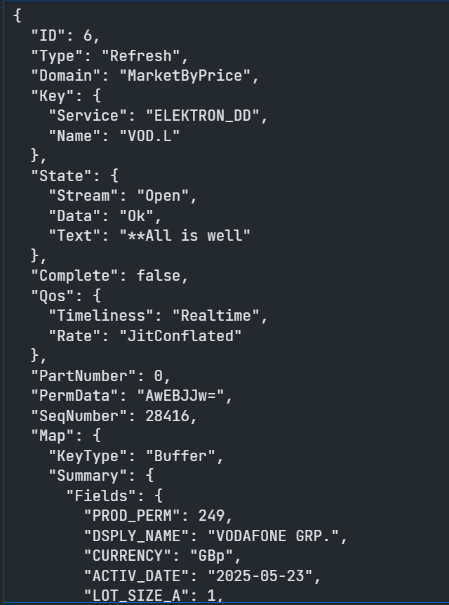
Assuming the request is valid, we should get back an Initial Refresh Msg representing the current state of the market for that instrument i.e. all open orders aggregated by price point.

At the start of the Refresh Msg you will see some header information including Summary Data - which contains non-order specific values like the Instrument name, the currency, most recent activity time, trading status, exchange ID and so on:

Following the Summary Data, you will receive the Order Book entries themselves:

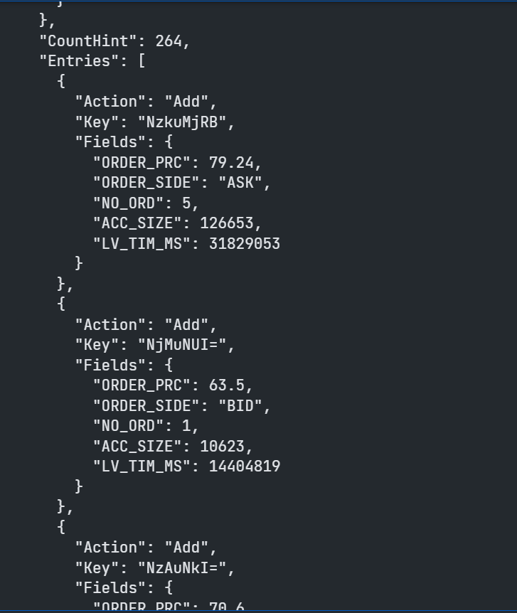
Here I have just pasted the first 3 of the 264 entries aggregated price points.

Once the complete Order Book has been delivered we can then expect to start receiving Update Msgs as the Market changes:

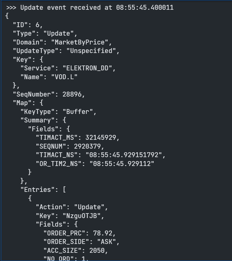
This Update Msg contains instructions to Update an existing Price Point in the Order Book. Update Msgs can also contain instructions to Add new Price points and/or Delete existing Price Points to/from the Order Book.

In addition to MarketByPrice data, the Delivery Layers will allow the consuming other Level 2 Streaming Domains - including any Custom Domain models published on your internal Real-Time Distribution System components (RDTS, formerly known as TREP).

There are much more examples of the Delivery Layer's Streaming object. Please find more details on the following resources:

Non-Streaming Data from the Delivery Platform

As well as Streaming Data, the Delivery layer will also allow you to access data normally delivered using the Request-Response mechanism such as Historical, Symbology, Fundamentals, Analytics, research, and so on.

Endpoint Interface

In the 1st part of this article, I mentioned that LSEG is gradually moving much of their vast breadth and depth of content onto the Delivery Platform.

Each unique content set will have its own Endpoint on the Delivery Data Platform - to access that content, you can do so use using the Endpoint interface provided as part of the Delivery Layer.

The Ownership Data

The Ownership API provides detailed information about a company's shareholders and holdings of investors/funds. This includes, Insider and Stakeholder Investors with capitalization summaries, a list of all Insider and Stakeholder stock owners, recent Buy and Sell activities, Top Concentrations on the stock.

Developers can use the Endpoint interface to access this data as follows:

Identify the Endpoint for Ownership data
Use the Endpoint Interface to send a request to the Endpoint
Decode the response and extract the Ownership data

Sounds simple enough, how does that work in practice?

Identifying the Endpoint

To ascertain the Endpoint, we can use the Data Platform's API Playground page - which an interactive documentation site you can access once you have a valid Data Platform account.

So, firstly we search for 'Ownership' to narrow down the list of Endpoints and then select the subset of the Ownership data that we are interested in, for example - consolidated investors:

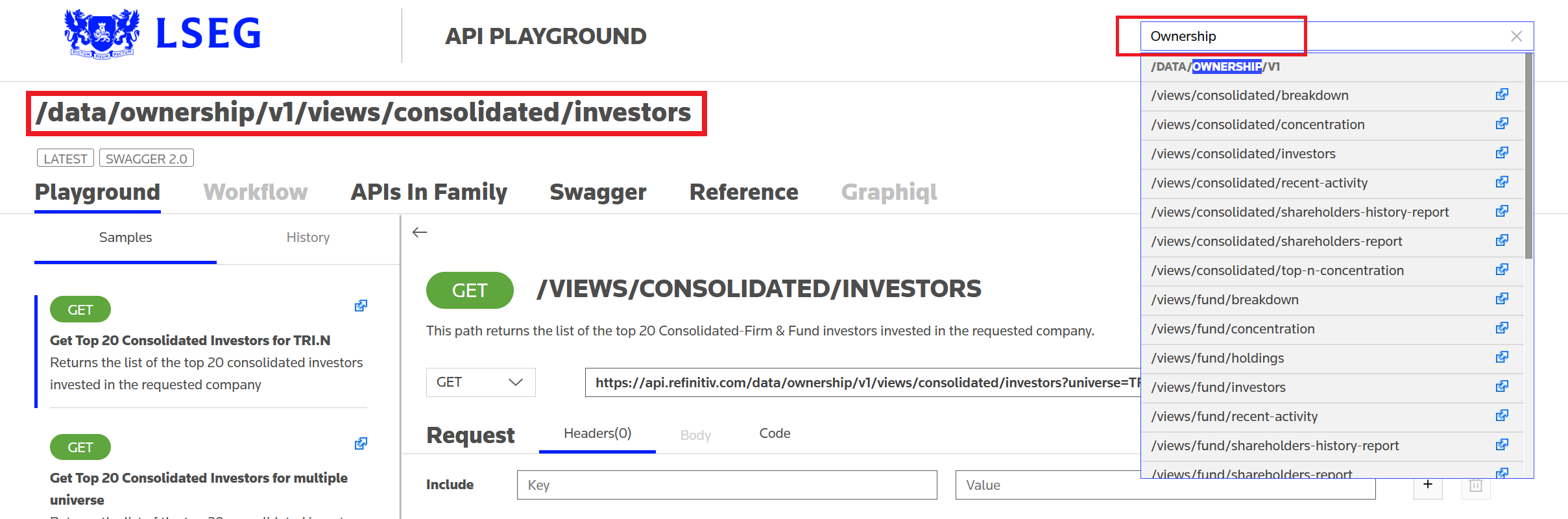
We then note the Endpoint URL - /data/ownership/v1/views/consolidated/investors - which can be used with the Endpoint interface as follows:

    	
            import lseg.data as ld
from lseg.data.delivery import endpoint_request
 
endpoint_url = "/data/ownership/v1/views/consolidated/investors"
request_definition = ld.delivery.endpoint_request.Definition(
    url = endpoint_url,
    method = ld.delivery.endpoint_request.RequestMethod.GET,
    query_parameters = {"universe": "LSEG.L"}
)
response = request_definition.get_data()
response.data.raw

We created the Endpoint object, passing in our session and the URL and then use the Endpoint to request the data for whatever entity we want - for example LSEG.L RIC code.

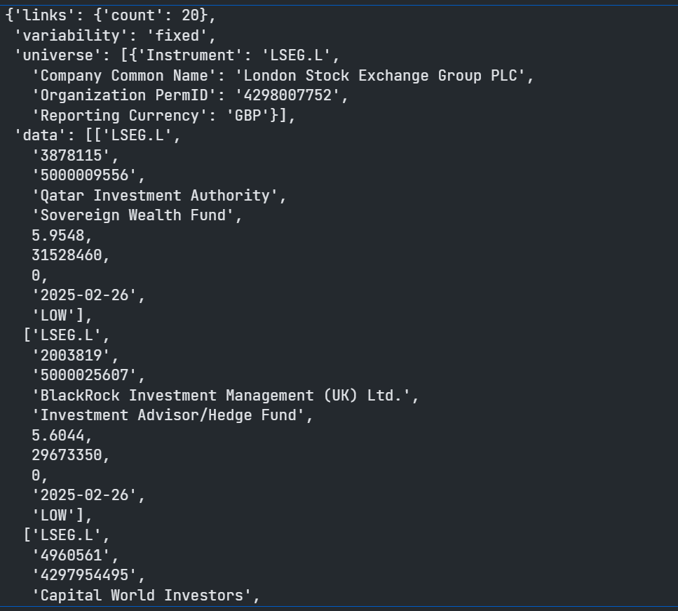
The payload is in JSON format that contains a list of LSEG.L top 20 investors.

You will, off course, find full documentation for each attribute on the API playground page - however, the JSON payload is self-describing and includes fairly verbose descriptions for the various scores at the end of the payload:

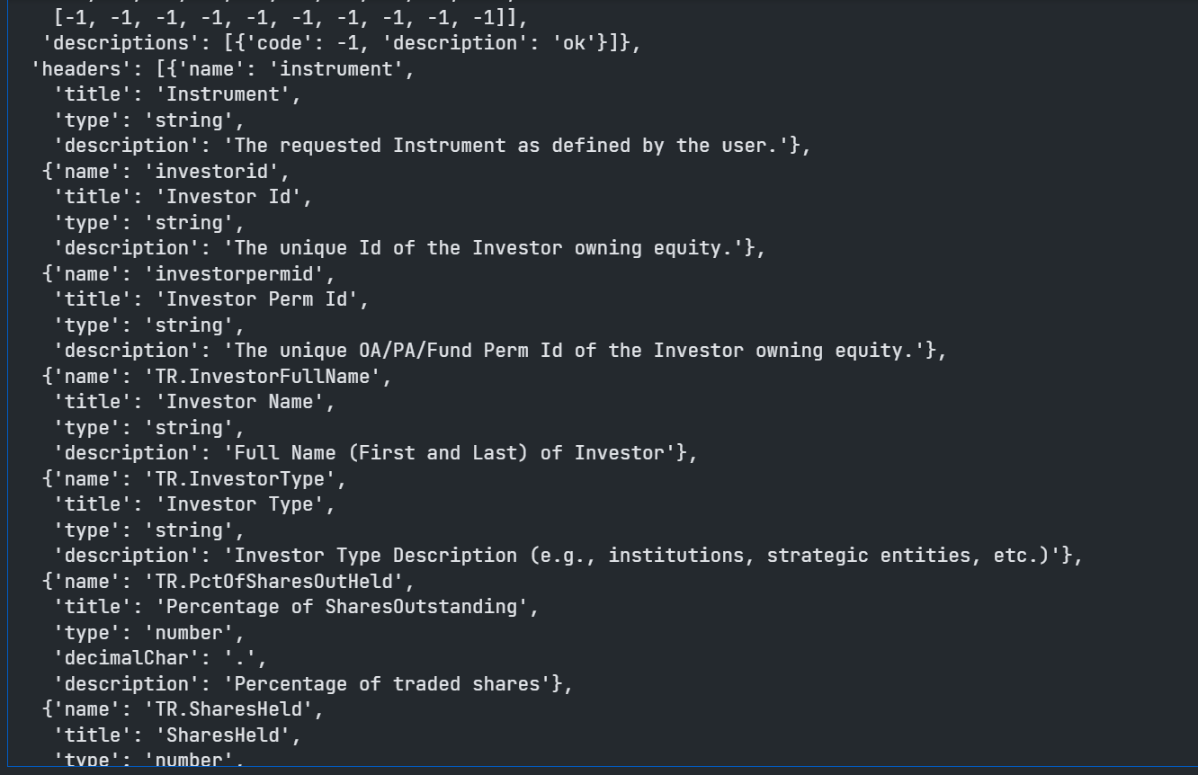
This saves us from having to cut and paste attribute names, descriptions etc from the documentation - instead we can just extract from the payload itself - particularly useful for GUI applications, displaying tooltips etc.

As the data is in JSON format, if we are working in Python, we can easily convert it to a Pandas DataFrame:

    	
            import pandas as pd
 
titles = [i["title"] for i in response.data.raw['headers']]
pd.DataFrame(response.data.raw['data'],columns=titles)

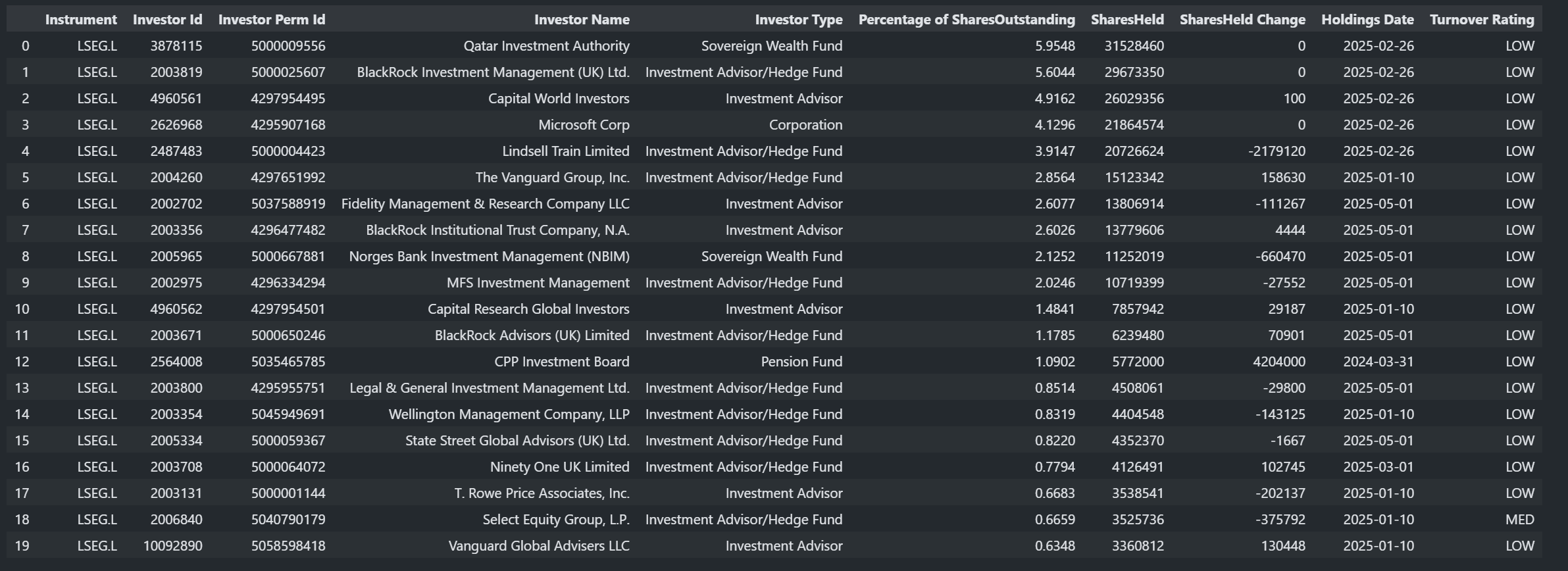
As you can see, even with the lowest level Delivery layer, it is still relatively straightforward to request advanced datasets and handle the response.

To illustrate this further, I would like to share a couple of other Endpoints that were demonstrated by one of my colleague's - Samuel Schwalm (Director, Enterprise Pricing Analytics) - at our recent London Developer Day event. I have picked these two Endpoints because I was amazed at just how easily you could access and display such rich data content. I expect that whilst you could do something similar in Excel, it would require much more effort and most likely involve several sheets of data, filters and Analytics functions.

Instrument Pricing Analytics - Volatility Surfaces Endpoint

The first example that Samuel showed us, used the Volatility Surfaces Endpoint.

Using the API Playground we can identify the Endpoint URL and create the Endpoint object:

    	
            from lseg.data.delivery import endpoint_request
import lseg.data as ld
import pandas as pd
import plotly.express as px
import plotly.graph_objects as go
import json
 
endpoint_url = 'https://api.refinitiv.com/data/quantitative-analytics-curves-and-surfaces/v1/surfaces'

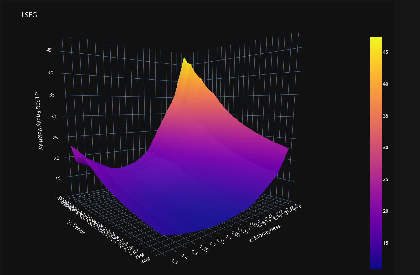
Then, using the reference documentation, we can build up our Request; Suppose we want to compare volatility for LSEG (LSEG.L) - we can generate a volatility surface:

from the Option Quote prices using an SSVI model
express the axes in Dates and Moneyness
and return the data in a matrix format
using the following request:

    	
            request_body={
            "universe": [
            {
                "surfaceTag": "LSEG",
                "underlyingType": "Eti",
                "underlyingDefinition": {
                    "instrumentCode": "LSEG.L"
                },
                "surfaceParameters": {
                    "inputVolatilityType": "Quoted",
                    "timeStamp": "Default",
                    "priceSide": "Mid",
                    "volatilityModel": "SVI",
                    "xAxis": "Tenor",
                    "yAxis": "Moneyness",
                    "calculationDate": "2025-05-20"
                },
                "surfaceLayout": {
                    "format": "Matrix",
                }
            }
            ],
        "outputs": ["Data", "ForwardCurve", "MoneynessStrike"]
}

And then we send the request to the Platform using HTTP POST method:

    	
            request_definition = ld.delivery.endpoint_request.Definition(
    method = ld.delivery.endpoint_request.RequestMethod.POST,
    url = endpoint_url,
    body_parameters = request_body
)
response = request_definition.get_data()

Once we get the response back, we can extract the payload and use the Plotly library to plot our data.

    	
            surface_tag = response.data.raw['data'][0]['surfaceTag']
 
_surface_df = pd.DataFrame(
    data=response.data.raw['data'][0]['surface'])
 
surface_df_title = f"{surface_tag} Equity Volatility Surface"
surface_df = pd.DataFrame(
    data=_surface_df.loc[1:,1:].values,
    index=_surface_df[0][1:],
    columns=_surface_df.iloc[0][1:])
surface_df.columns.name = "Moneyness"
surface_df.index.name = "Tenor"
 
surface_plot_df = surface_df
 
fig = go.Figure(data=[go.Surface(z=surface_plot_df.values)])
 
fig.update_layout(
    template="plotly_dark",
    title=surface_tag,
    autosize=False,
    width=1000, height=700,
    margin=dict(l=5, r=5, b=5, t=80),
    scene=dict(
        aspectratio =  {"x": 1, "y": 1, "z": 1},
        xaxis_title=f"x: {surface_plot_df.columns.name}",
        yaxis_title=f"y: {surface_plot_df.index.name}",
        zaxis_title=f"z: {surface_tag} Equity Volatility",
        xaxis=dict(ticktext=list(surface_plot_df.columns),
                   tickvals=[i for i in range(len(surface_plot_df.columns))]),
        yaxis=dict(ticktext=list(surface_plot_df.index),
                   tickvals=[i for i in range(len(surface_plot_df))]),
    ))
 
fig.show()

Resulting in our lovely Surface plot:

Instrument Pricing Analytics - Zero-Coupon Curves Endpoint

Another example that Samuel showed us during the London Developer day, used the Zero-Coupon Endpoint.

Using the API Playground documentation, we again determine the Endpoint URL, create the Endpoint object, build our request and send it to the Platform. If we wanted to ask for:

the swap-derived zero curves for the available EURIBOR tenors (1M, 3M, 6M)
zc curves to be generated using an OIS discounting methodology
mid swap market quotes to be used
interpolation using cubic spline
and any extrapolation to be done in a linear way

We would send the following request:

    	
            endpoint_url = 'https://api.refinitiv.com/data/quantitative-analytics-curves-and-surfaces/v1/curves/zc-curves'
 
request_body = {
  "universe": [
    {
      "curveDefinition": {
        "currency": "EUR",
        "indexName": "EURIBOR",
        "name": "EUR EURIBOR Swap ZC Curve",
        "source": "Refinitiv",
        "discountingTenor": "OIS"
      }
    }
  ]
}
 
response =  ld.delivery.endpoint_request.Definition(
    method = ld.delivery.endpoint_request.RequestMethod.POST,
    url = endpoint_url,
    body_parameters = request_body
).get_data()

We can then use the payload response to display the curves (using Matplotlib Pyplot) generated for the 1M, 3M and 6M Eurobor swap as well as the EONIA cz curve used for discounting:

    	
            import matplotlib.pyplot as plt
 
def plot_zc_curves(curves, curve_tenors=None, smoothingfactor=None):
    tenors = curve_tenors if curve_tenors!=None else curves['description']['curveDefinition']['availableTenors'][:-1]
   
    s = smoothingfactor if smoothingfactor != None else 0.0
    fig = plt.figure(figsize=[30,10])
    ax = plt.axes()
   
    ax.set_xlabel('time')
    ax.set_ylabel('zc rate')
    title = 'zc Curves'
   
    ax.set_title(title)
    for tenor in tenors:
        curve = pd.DataFrame(data=curves['curves'][tenor]['curvePoints'])
        x = convert_ISODate_to_float(curve['endDate'])
        y = curve['ratePercent']
        xnew, ynew = smooth_line(x,y,100,s)
        ax.plot(xnew,ynew,label=tenor)
   
    plt.xticks(rotation='vertical')
    plt.legend()
    plt.show()
   
def convert_ISODate_to_float(date_string_array):
    import datetime
    import matplotlib.dates as dates
   
    date_float_array = []
    for date_string in date_string_array:
        date_float = dates.date2num(datetime.datetime.strptime(date_string, '%Y-%m-%d'))
        date_float_array.append(date_float)
    return date_float_array
 
def smooth_line(x, y, nb_data_points, smoothing_factor=None):
   
    import scipy.interpolate as interpolate
    import numpy as np
    import math as math
 
    s = 0.0 if (smoothing_factor==0.0) else len(x) + (2 * smoothing_factor - 1) * math.sqrt(2*len(x))
 
    t,c,k = interpolate.splrep(x,y,k=3,s=s)
   
    xnew = np.linspace(x[0], x[-1], nb_data_points)
    spline =  interpolate.BSpline(t, c, k, extrapolate=False)
   
    xnew = np.linspace(x[0], x[-1], nb_data_points)
    ynew = spline(xnew)
 
    return xnew, ynew
 
curves = response.data.raw['data'][0]
plot_zc_curves(curves, ['1M','3M','6M','OIS'])

Which should produce something that looks like this:

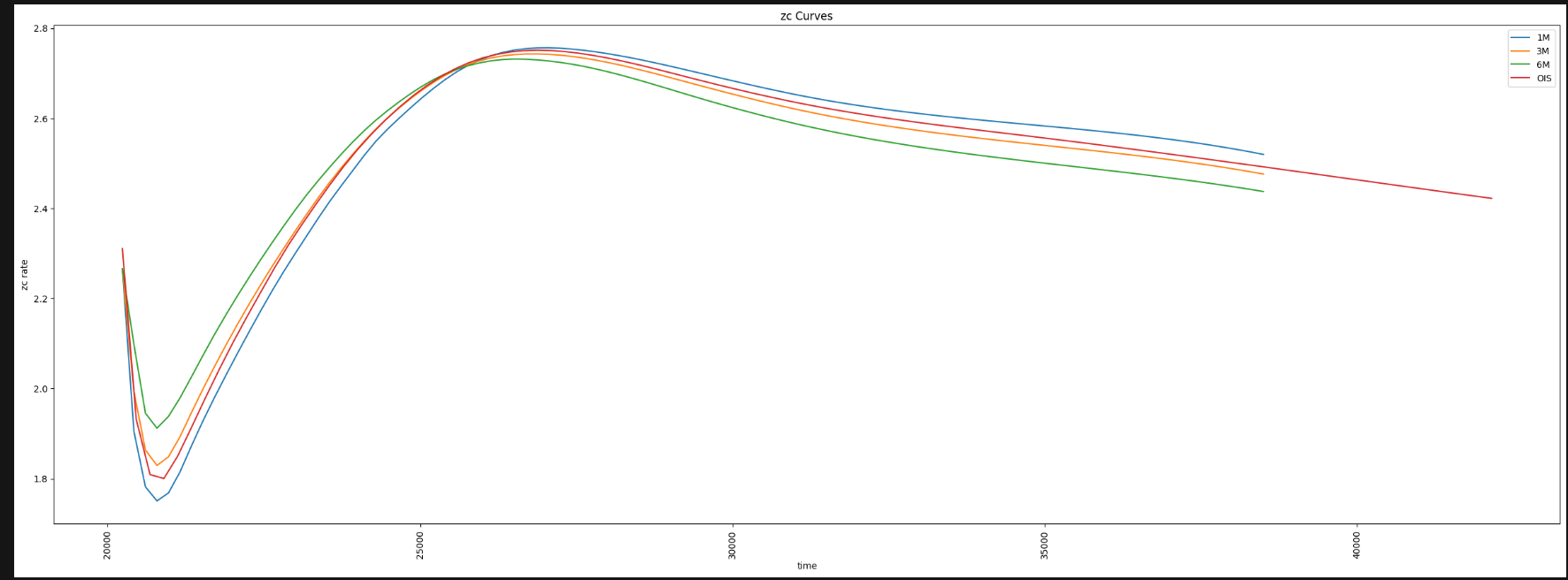
Based on the examples above, I hope you will agree, that the Analytics Endpoints are incredibly versatile and powerful allowing you to perform complex analysis on the Platform using the latest market contributions in a straightforward yet flexible manner.

Additional Endpoints

At the time of writing, there are ton of other Endpoints available on the Delivery Platform including, but not limited to:

Alerts subscriptions for Research data, News and Headlines
Company Fundamentals - such a Balance sheet, Cash flow, financial summary etc
Symbology - symbol lookup to and from different symbology types (The Content Layer has this interface)
Ultimate Beneficial Ownership
Search - simple and structured (The Access and Content Layers have this interface)
Aggregates - e.g. Business Classifications
Client File Store
Filings
Bulk Search
Event Calendar