
Author:

This article and sample code demonstrate how to use the LSEG Data Library for Python to calculate Normal Beta, Beta Up, and Beta Down for any company and index on any given date, following the methodology outlined in the Company Beta Types – Historical Workspace Excel template.

This methodology incorporates different parameters for each type of Beta, including the calculation range and the periodicity of the data.
- Normal Beta measures a security’s volatility relative to the overall market.
- Beta Up measures a security’s volatility relative to the market, but only on days when the benchmark’s return is positive.
- Beta Down measures a security’s volatility relative to the market, but only on days when the benchmark’s return is negative.

| Normal Beta | Beta Up | Beta Down |
|---|---|---|
| A measure of the stock price volatility relative to the benchmark market. It is a covariance of the security’s price movement in relation to the market’s price movement. Beta is calculated using the least squares linear regression formula. | A measure of the stock price volatility relative to the benchmark market. It is a covariance of the security’s price movement in relation to the market’s price movement. Beta Up is calculated using the least squares linear regression formula and only uses positive price points. | A measure of the stock price volatility relative to the benchmark market. It is a covariance of the security’s price movement in relation to the market’s price movement. Beta Down is calculated using the least squares linear regression formula and only uses negative price points. |
| An Up data point is defined as a period when the benchmark is up. | A Down data point is defined as a period when the benchmark is down. | |
| Benchmark is set based on the primary exchange the security trade. | Benchmark is set based on the primary exchange the security trade. | Benchmark is set based on the primary exchange the security trade. |
Available periods:
|
Available periods:
|
Available periods:
|
| Calculation of Beta requires a certain number of data points to be available. A data point consists of a percentage change for the stock and the benchmark, for the same time period. Time periods are non-overlapping, and the weekly and monthly sample sets roll ahead at the beginning of each new week or month. | Calculation of Beta requires a certain number of data points to be available. A data point consists of a percentage change for the stock and the benchmark, for the same time period. Time periods are non-overlapping, and the weekly and monthly sample sets roll ahead at the beginning of each new week or month. | Calculation of Beta requires a certain number of data points to be available. A data point consists of a percentage change for the stock and the benchmark, for the same time period. Time periods are non-overlapping, and the weekly and monthly sample sets roll ahead at the beginning of each new week or month. |
Calculation of Beta requires at least 2/3 of non-null data points to be present.
NULL/empty value will appear if minimum data points requirement are not met. |
Up calculation of Beta require at least 1/6 of data points to be present.
NULL/empty value will appear if minimum data points requirement are not met. |
Down calculation of Beta require at least 1/6 of data points to be present.
NULL/empty value will appear if minimum data points requirement are not met. |
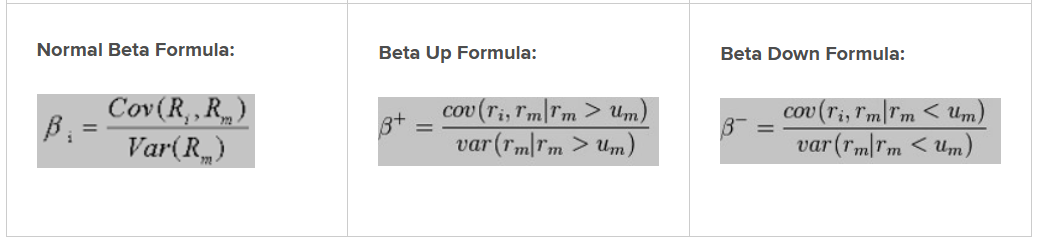
Formula
Required Inputs
- Company Code (RIC): Ticker (RIC) of the subject company.
- Index Code (RIC): Ticker (RIC) of the subject index.
- Historical Date:The end-date for querying events.
Calculation
The following steps are used to calculate the Company Beta Types - Historical.
| Steps | Descriptions |
|---|---|
| Step 1 | Price series of the Stock and Index |
| Step 2 | Calculation of return from the stock and index |
| Step 3 | Exclusion of values that are not negative or positive from the index return series |
| Step 4 | Series of negative or positive Index Return |
| Step 5 | Calculation of BETA's value |
Python Code
The sample code imports and uses the following Python libraries:
- lseg.data: Provides high‑level APIs for accessing market data—such as prices, fundamentals, and news—from LSEG platforms (for example, the Data Platform and Workspace).
- lseg.data.content.historical_pricing: Exposes the historical pricing endpoint, which enables access to time‑series price data (such as OHLC, closing prices, and volume) for instruments identified by symbols or identifiers like RICs
- NumPy: Supports numerical computing with arrays and vectorized mathematical operations.
- Pandas: Provides Series and DataFrame structures for working with tabular and time‑series data, making it well suited for pricing data analysis, resampling, joins, and rolling calculations.
Then, the code calls the ld.open_session() method to establish a connection to the Workspace desktop session.
import lseg.data as ld
from lseg.data.content import historical_pricing
import numpy as np
import pandas as pd
import warnings
warnings.simplefilter(action='ignore', category=FutureWarning)
pd.set_option('future.no_silent_downcasting', True)
ld.open_session()
Step 1: Price series of the Stock and Index
The function defined for this step accepts the following parameters:
- ric (str): The stock RIC.
- index (str): The index RIC.
- interval (str): An interval string for filtering historical pricing events, such as P1D (daily), P1W (weekly), and P1M (monthly)ใ
- end (str): The end-date string for querying events, formatted as YYYY‑MM‑DD.
- datapoints (int): A maximum number of rows to return.
It will return a data frame.
This function uses the historical_pricing endpoint to retrieve historical close pricings for both the stock and the index. It then merges the results into a single DataFrame and returns it to the caller.
def Step1(ric: str, index: str, interval: str, end: str, datapoints: int) -> pd.DataFrame:
stock_resp = historical_pricing.summaries.Definition(
ric,
interval=interval,
end = end,
count = datapoints,
fields=['TRDPRC_1'],
extended_params={"includeTradeIndicator":"True"}
).get_data()
stock_df = stock_resp.data.df.ffill()
if 'TRADE_IND' in stock_df.columns:
stock_df = stock_df.drop(['TRADE_IND'], axis=1)
stock_reverse = stock_df.iloc[::-1]
#Index
index_resp = historical_pricing.summaries.Definition(
index,
interval=interval,
end = end,
count = datapoints,
fields=['TRDPRC_1'],
extended_params={"includeTradeIndicator":"True"}
).get_data()
index_df = index_resp.data.df.ffill()
if 'TRADE_IND' in index_df.columns:
index_df = index_df.drop(['TRADE_IND'], axis=1)
index_reverse = index_df.iloc[::-1]
df = stock_reverse.copy()
df.columns = ['Stock Trade Close']
df['Index Trade Close'] = index_reverse['TRDPRC_1']
return df
Example
The function can be called like this:
| Step1_df = Step1('PTT.BK','.SETI', 'P1D', '2026-01-23', 91) |
Step1_df = Step1('PTT.BK','.SETI', 'P1D', '2026-01-23', 91)
Step1_df
The output is:
| Stock Trade Close | Index Trade Close | |
|---|---|---|
| Date | ||
| 2026-01-23 | 33.75 | 1314.39 |
| 2026-01-22 | 33.75 | 1311.64 |
| 2026-01-21 | 33.5 | 1317.56 |
| 2026-01-20 | 33.75 | 1296.37 |
| 2026-01-19 | 33.25 | 1283.2 |
| ... | ... | ... |
| 2025-09-25 | 33.25 | 1288.26 |
| 2025-09-24 | 33.0 | 1278.41 |
| 2025-09-23 | 33.0 | 1273.2 |
| 2025-09-22 | 33.0 | 1282.54 |
| 2025-09-19 | 33.25 | 1292.72 |
91 rows × 2 columns
Step 2: Calculation of return from the stock and index
The function defined for this step takes the data frame produced in the first step as input. It uses the close prices from that data frame to calculate the returns for both the stock and the index, and then returns a new data frame to the caller.
def Step2(input_df: pd.DataFrame) -> pd.DataFrame:
#Calculate Stock Return
stock_df = pd.DataFrame(input_df['Stock Trade Close'])[::-1]
stock_reverse1 = stock_df.shift()[::-1]
stock1 = np.log(stock_df / stock_reverse1)
stock1 = stock1.dropna()
step2 = stock1.copy()
step2.columns = ['Stock Return']
#Calculate Index Return
index_df = pd.DataFrame(input_df['Index Trade Close'])[::-1]
index_reverse1 = index_df.shift()[::-1]
index1 = np.log(index_df / index_reverse1)
index1 = index1.dropna()
step2['Index Return']=index1['Index Trade Close']
return step2[::-1]
Example
The function can be called like this:
| Step2_df = Step2(Step1_df) |
Step2_df = Step2(Step1_df)
Step2_df
The output is:
| Stock Return | Index Return | |
|---|---|---|
| Date | ||
| 2026-01-23 | 0.0 | 0.002094 |
| 2026-01-22 | 0.007435 | -0.004503 |
| 2026-01-21 | -0.007435 | 0.016213 |
| 2026-01-20 | 0.014926 | 0.010211 |
| 2026-01-19 | 0.007547 | 0.00594 |
| ... | ... | ... |
| 2025-09-26 | 0.0 | -0.007417 |
| 2025-09-25 | 0.007547 | 0.007675 |
| 2025-09-24 | 0.0 | 0.004084 |
| 2025-09-23 | 0.0 | -0.007309 |
| 2025-09-22 | -0.007547 | -0.007906 |
90 rows × 2 columns
Step 3: Exclusion of values that are not negative or positive from the index return series
The function defined for this step accepts the data frame produced in the second step, along with the calculation method to be applied.
- input_df (pd.DataFrame): The data frame generated from the second step.
- beta (str): The calculation method used to compute the beta value. Valid options include '', 'up', or 'down'.
If the calculation method is 'up', all zero and negative index returns are replaced with NaN.
If the calculation method is 'down', all zero and positive index returns are replaced with NaN.
If the calculation method is the normal mode (''), a copy of the input data frame is returned unchanged.
def Step3(input_df: pd.DataFrame, beta: str = '') -> pd.DataFrame:
step3 = pd.DataFrame()
if beta.lower()=='up':
step3['Stock Return'] = input_df['Stock Return']
step3['Only Positive Index Return'] = input_df.apply(lambda x: np.nan if x['Index Return'] <= 0 else x['Index Return'],axis=1)
#step3 = step3.dropna()
elif beta.lower()=='down':
step3['Stock Return'] = input_df['Stock Return']
step3['Only Negative Index Return'] = input_df.apply(lambda x: np.nan if x['Index Return'] >= 0 else x['Index Return'],axis=1)
#temp = temp.dropna()
else:
return input_df.copy()
return step3
Examples
The function can be called like this:
Normal Beta
| Step3_df = Step3(Step2_df, '') |
Beta Up
| Step3_df = Step3(Step2_df, 'up') |
Beta Down
| Step3_df = Step3(Step2_df, 'down') |
Step3_df = Step3(Step2_df, 'up')
Step3_df
The output is:
| Stock Return | Only Positive Index Return | |
|---|---|---|
| Date | ||
| 2026-01-23 | 0.0 | 0.002094 |
| 2026-01-22 | 0.007435 | NaN |
| 2026-01-21 | -0.007435 | 0.016213 |
| 2026-01-20 | 0.014926 | 0.010211 |
| 2026-01-19 | 0.007547 | 0.005940 |
| ... | ... | ... |
| 2025-09-26 | 0.0 | NaN |
| 2025-09-25 | 0.007547 | 0.007675 |
| 2025-09-24 | 0.0 | 0.004084 |
| 2025-09-23 | 0.0 | NaN |
| 2025-09-22 | -0.007547 | NaN |
90 rows × 2 columns
Step 4: Series of negative or positive Index Return
The function defined for this step takes the data frame produced in the third step, removes all unavailable data, and returns the cleaned data frame to the caller.
def Step4(input_df: pd.DataFrame) -> pd.DataFrame:
return input_df.dropna()
Example
The function can be called like this:
| Step4_df = Step4(Step3_df) |
Step4_df = Step4(Step3_df)
Step4_df
The output is:
| Stock Return | Only Positive Index Return | |
|---|---|---|
| Date | ||
| 2026-01-23 | 0.0 | 0.002094 |
| 2026-01-21 | -0.007435 | 0.016213 |
| 2026-01-20 | 0.014926 | 0.010211 |
| 2026-01-19 | 0.007547 | 0.005940 |
| 2026-01-16 | 0.007605 | 0.011202 |
| ... | ... | ... |
| 2025-10-02 | 0.0 | 0.010346 |
| 2025-10-01 | -0.030537 | 0.000675 |
| 2025-09-29 | 0.014926 | 0.007270 |
| 2025-09-25 | 0.007547 | 0.007675 |
| 2025-09-24 | 0.0 | 0.004084 |
90 rows × 2 columns
Step 5: Calculation of BETA's value
The function defined for this step uses the data frame produced in the fourth step to calculate a beta value.
It applies the numpy.polyfit function to estimate the relationship between stock returns and index returns—a common approach for computing beta in finance. The function passes the stock returns as the first argument (the x-coordinates of the sample points), the index returns as the second argument (the y-coordinates), and 1 as the third argument to indicate a first‑degree polynomial fit.
The function then returns the first value produced by numpy.polyfit, which corresponds to the slope of the fitted line.
def Step5(input_df: pd.DataFrame):
slope, _ = np.polyfit(
x=input_df.iloc[:, 1].tolist(),
y=input_df.iloc[:,0].tolist(),
deg=1)
return slope
Example
The function can be called like this:
| Beta_value = Step5(Step4_df) |
Beta_value = Step5(Step4_df)
Beta_value
The output is:
np.float64(0.5307264916476)
Usage
To use these functions, you must define a list of parameters used to calculate beta values. Each entry includes the following properties:
- Name: The name of Beta value
- Periodicity: An interval string for filtering historical pricing events, such as P1D (daily), P1W (weekly), and P1M (monthly)
- Data Points: A maximum number of rows to return
- Rule of % Available: A percentage number of data points to be available for calculation
- Calculation Method: The calculation method used to compute the beta value. Valid options include '', 'up', or 'down'
The following code defines 11 rules used to calculate beta values.
beta_data = [
{
'Name':'Beta - 90 Days - Daily',
'Periodcity':'P1D',
'Data Points':91,
'Rule of % Avaialble': 67,
'Calculation Method': ''
},
{
'Name':'Beta - 181 Days - Daily',
'Periodcity':'P1D',
'Data Points':181,
'Rule of % Avaialble': 67,
'Calculation Method': ''
},
{
'Name':'Beta - 2 Years - Weekly',
'Periodcity':'P1W',
'Data Points':105,
'Rule of % Avaialble': 67,
'Calculation Method': ''
},
{
'Name':'Beta - 3 Years - Weekly',
'Periodcity':'P1W',
'Data Points':157,
'Rule of % Avaialble': 67,
'Calculation Method': ''
},
{
'Name':'Beta - 5 Years - Monthly',
'Periodcity':'P1M',
'Data Points':61,
'Rule of % Avaialble': 67,
'Calculation Method': ''
},
{
'Name':'Beta Up - 2 Years - Weekly',
'Periodcity':'P1W',
'Data Points':105,
'Rule of % Avaialble': 17,
'Calculation Method': 'up'
},
{
'Name':'Beta Up - 3 Years - Weekly',
'Periodcity':'P1W',
'Data Points':157,
'Rule of % Avaialble': 17,
'Calculation Method': 'up'
},
{
'Name':'Beta Up - 5 Years - Monthly',
'Periodcity':'P1M',
'Data Points':61,
'Rule of % Avaialble': 17,
'Calculation Method': 'up'
},
{
'Name':'Beta Down - 2 Years - Weekly',
'Periodcity':'P1W',
'Data Points':105,
'Rule of % Avaialble': 17,
'Calculation Method': 'down'
},
{
'Name':'Beta Down - 3 Years - Weekly',
'Periodcity':'P1W',
'Data Points':157,
'Rule of % Avaialble': 17,
'Calculation Method': 'down'
},
{
'Name':'Beta Down - 5 Years - Monthly',
'Periodcity':'P1M',
'Data Points':61,
'Rule of % Avaialble': 17,
'Calculation Method': 'down'
}
]
beta_table = pd.DataFrame(beta_data)
beta_table
The output is:
| Name | Periodcity | Data Points | Rule of % Avaialble | Calculation Method | |
|---|---|---|---|---|---|
| 0 | Beta - 90 Days - Daily | P1D | 91 | 67 | |
| 1 | Beta - 181 Days - Daily | P1D | 181 | 67 | |
| 2 | Beta - 2 Years - Weekly | P1W | 105 | 67 | |
| 3 | Beta - 3 Years - Weekly | P1W | 157 | 67 | |
| 4 | Beta - 5 Years - Monthly | P1M | 61 | 67 | |
| 5 | Beta Up - 2 Years - Weekly | P1W | 105 | 17 | up |
| 6 | Beta Up - 3 Years - Weekly | P1W | 157 | 17 | up |
| 7 | Beta Up - 5 Years - Monthly | P1M | 61 | 17 | up |
| 8 | Beta Down - 2 Years - Weekly | P1W | 105 | 17 | down |
| 9 | Beta Down - 3 Years - Weekly | P1W | 157 | 17 | down |
| 10 | Beta Down - 5 Years - Monthly | P1M | 61 | 17 | down |
Next, define a function that iterates through all entries in the list and calculates the beta values for each one. The function accepts the following parameters:
- input_df (pd.DataFrame): The data frame containing the rules for calculating beta values.
- ric (str): The stock RIC.
- index (str): The index RIC.
- end (str): The end-date string for querying events, formatted as YYYY‑MM‑DD.
This function invokes the methods defined in Steps 1 through 5 and returns a data frame containing the resulting beta values.
def CalculateBeta(input_df: pd.DataFrame, ric: str, index: str, end: str) -> pd.DataFrame:
column_names = [
'Name',
'Numbers of Stocks Returns',
'Numbers of Stocks Returns, relative to Beta Analysis',
'% of data results',
'Rule of % Available',
'Results Analysis',
'Values']
summary_df = pd.DataFrame(columns=column_names)
for i, row in input_df.iterrows():
step1_df = Step1(ric, index, row['Periodcity'], end, row['Data Points'])
#display(step1_df)
step2_df = Step2(step1_df)
#display(step2_df)
step3_df = Step3(step2_df, row['Calculation Method'])
#display(step3_df)
step4_df = Step4(step3_df)
#display(step4_df)
step5 = Step5(step4_df)
if row['Calculation Method'] == '':
summary_df.loc[len(summary_df)]=[row['Name'],len(step2_df),None, None, row['Rule of % Avaialble'], None, step5]
else:
summary_df.loc[len(summary_df)]=[row['Name'],len(step2_df),len(step4_df), (len(step4_df) / len(step2_df))*100, row['Rule of % Avaialble'], 'Beta Valid' if (len(step4_df) / len(step2_df))*100 >= row['Rule of % Avaialble'] else 'Beta Invalid' , step5]
return summary_df
Example
The function can be called like this:
| ric = 'PTT.BK' index = '.SETI' end = '2026-01-23' CalculateBeta(beta_table, ric, index, end) |
from datetime import datetime
ric = 'PTT.BK'
index = '.SETI'
end = datetime.today().strftime('%Y-%m-%d')
CalculateBeta(beta_table, ric, index, end)
The output is:
| Name | Numbers of Stocks Returns | Numbers of Stocks Returns, relative to Beta Analysis | % of data results | Rule of % Available | Results Analysis | Values | |
|---|---|---|---|---|---|---|---|
| 0 | Beta - 90 Days - Daily | 90 | None | NaN | 67 | None | 0.563929 |
| 1 | Beta - 181 Days - Daily | 180 | None | NaN | 67 | None | 0.585150 |
| 2 | Beta - 2 Years - Weekly | 104 | None | NaN | 67 | None | 0.615219 |
| 3 | Beta - 3 Years - Weekly | 156 | None | NaN | 67 | None | 0.638245 |
| 4 | Beta - 5 Years - Monthly | 60 | None | NaN | 67 | None | 0.689380 |
| 5 | Beta Up - 2 Years - Weekly | 104 | 49 | 47.115385 | 17 | Beta Valid | 0.500292 |
| 6 | Beta Up - 3 Years - Weekly | 156 | 73 | 46.794872 | 17 | Beta Valid | 0.570310 |
| 7 | Beta Up - 5 Years - Monthly | 60 | 30 | 50.000000 | 17 | Beta Valid | 0.943862 |
| 8 | Beta Down - 2 Years - Weekly | 104 | 55 | 52.884615 | 17 | Beta Valid | 0.437878 |
| 9 | Beta Down - 3 Years - Weekly | 156 | 83 | 53.205128 | 17 | Beta Valid | 0.499133 |
| 10 | Beta Down - 5 Years - Monthly | 60 | 30 | 50.000000 | 17 | Beta Valid | 0.475566 |
Summary
The article provides a step‑by‑step translation of the Workspace Excel formulas used in the Company Beta Types – Historical Excel template into Python code. Its primary goal is to demonstrate how to compute three key beta measures—Normal Beta, Beta Up, and Beta Down—for any selected company and benchmark index on any specified date.
To achieve this, the article leverages the LSEG Data Library for Python, which serves as the data‑access layer for retrieving historical closing prices for both the target stock and its corresponding index. Once the historical price series is obtained, the workflow proceeds by transforming the prices into return series, typically using daily percentage changes or log returns, depending on the analytical convention.
After constructing the return series for both the stock and the index, the article explains how to apply the same logic embedded in the Excel template to compute the different beta types. Normal Beta is derived from the covariance of stock and index returns relative to the variance of index returns. Beta Up and Beta Down are calculated using return subsets filtered on whether index returns are positive or negative, respectively—mirroring the conditional calculations performed in the Workspace Excel template.
By walking through each stage of the process—from data retrieval to return transformation to beta estimation—the article not only replicates the Excel workflow but also illustrates how these computations can be automated, reproduced, and scaled in Python for broader analytical applications.
Get In Touch
Related APIs
Source Code
Related Articles
-
Time Series Forecasting with Data Library for Python
-
Using Economic Indicators with Eikon Data API - A Machine Learning Example
-
Inflation versus Dollar Cost Averaging on Pension Fund with Data Library
-
Create Technical Analysis triggers and signals using the LSEG Data Library for Python
-
Peer Analysis