ime Series Forecasting with Data Library for Python

April 10,2025

Pimchaya Wongrukun

Wasin Waeosri

Overview

Last Updated: April 2025

This article demonstrates how to extract the time series from LSEG Workspace platform using Data Library for Python (LSEG Data Library, aka Data Library version 2). Then, we can use it for forecasting the time series e.g. using ARIMA (Autoregressive integrated moving average) models in an example notebook application.

Introduction to the Data Library for Python

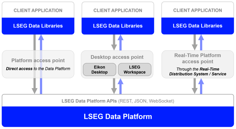
Let me start by give you an introduction to the Data Library. The Data Library for Python provides a set of ease-of-use interfaces offering coders uniform access to the breadth and depth of financial data and services available on the Workspace, RDP, and Real-Time Platforms. The API is designed to provide consistent access through multiple access channels and target both Professional Developers and Financial Coders. Developers can choose to access content from the desktop, through their deployed streaming services, or directly to the cloud. With the Data Library, the same Python code can be used to retrieve data regardless of which access point you choose to connect to the platform.

The Data Library are available in the following programming languages:

For more deep detail regarding the Data Library for Python, please refer to the following articles and tutorials:

Disclaimer

This article is based on Data Library Python versions 2.1.1 using the Desktop Session only.

That covers an overview of the Data Library

Introduction to ARIMA models

My next point is the ARIMA model. The ARIMA models are a class of statistical models for analyzing and forecasting time series data. ARIMA consists of the following key aspects of the model

AR: Autoregression. A model that uses the dependent relationship between an observation and some number of lagged observations.
I: Integrated. The use of differencing of raw observations (e.g. subtracting an observation from an observation at the previous time step) in order to make the time series stationary.
MA: Moving Average. A model that uses the dependency between an observation and a residual error from a moving average model applied to lagged observations.

Each of these components are explicitly specified in the model as a parameter. A standard notation is used of ARIMA(p,d,q) where the parameters are substituted with integer values to quickly indicate the specific ARIMA model being used.

The parameters of the ARIMA model are defined as follows:

p: The number of lag observations included in the model, also called the lag order.
d: The number of times that the raw observations are difference, also called the degree of differencing.
q: The size of the moving average window, also called the order of moving average.

A value of 0 can be used for a parameter, which indicates to not use that element of the model. This way, the ARIMA model can be configured to perform the function of an ARMA model, and even a simple AR, I, or MA model.

That’s all I have to say about the ARIMA models.

Prerequisite

The example project application requires the following dependencies.

LSEG Workspace desktop application with access to Data Library for Python.
Python (Ananconda or MiniConda distribution/package manager also compatible).
Jupyter Lab application.

Note:

The example project has been qualified with Python version 3.11.5
If you are not familiar with Jupyter Lab application, the following tutorial created by DataCamp may help you.

Code Walkthrough

Let start with importing the required libraries. The application needs to import lseg.data, matplotlib, pandas, and numpy library in order to interact with Data library, DataFrame object and plot graph.

    	
            import lseg.data as ld
import pandas as pd
import matplotlib
import matplotlib.pyplot as plt
import numpy as np
import warnings

The next step is to open a session defined in a lseg-data.config.json configuration file in the same location as an application file.

You should save a json file lseg-data.config.json having your Workspace App Key as follows:

    	
            {
    "logs": {
        "level": "debug",
        "transports": {
            "console": {
                "enabled": false
            },
            "file": {
                "enabled": false,
                "name": "lseg-data-lib.log"
            }
        }
    },
    "sessions": {
        "default": "desktop.workspace",
        "desktop": {
            "workspace": {
                "app-key": "YOUR APP KEY GOES HERE!"
            }
        }
    }
}

This file should be readily available (e.g. in the current working directory) for the next steps.

Please note that the LSEG Workspace desktop application integrates the API proxy that acts as an interface between the Data library and the Workspace Platform. For this reason, the Workspace application must be running when you use the Data library with Desktop Session.

Open the data session

The open_session() function creates and open sessions based on the information contained in the lseg-data.config.json configuration file. Please edit this file to set the session type and other parameters required for the session you want to open.

    	
            ld.open_session()
# example output <lseg.data.session.Definition object at xxxx {name='workspace'}>

The Data Library provides get_history() function to access pricing history as well as Fundamental & Reference data history via a single function call.

You can use the Python built-in help() function or Reference Guide document to check the parameters options in detail.

    	
            help(ld.get_history)

The get_history() function returns a pandas.DataFrame. It raises exceptions on error and when no data is available. Please check out the Usage and Limits Guideline document.

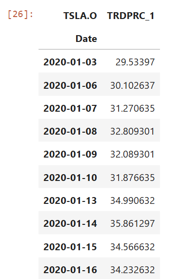
I am demonstrating with TESLA company (RIC Code: TSLA.O).

    	
            ric = 'TSLA.O'
start_date = '2020-01-02'
fields = ['TRDPRC_1']
 
df = ld.get_history(
    universe=ric,
    fields=fields,
    interval='daily',
    start=start_date,
    count = 10000)
df.head(10)

Result:

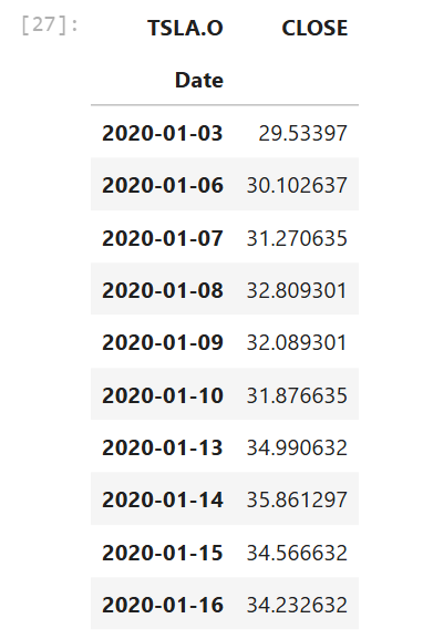
To make our DataFrame easier to read, I am changing a column name from TRDPRC_1 to be CLOSE to represent the close price of each day.

    	
            df.rename(
    columns= {
        'TRDPRC_1':'CLOSE'
    },
    inplace= True
)
df.head(10)

That is all for the data preparation process. We can close the session with Workspace now.

    	
            ld.close_session()

Now, what about the ARIMA models? To use the ARIMA models, you need to import the statsmodels Python library to use the models in an application.

    	
            from statsmodels.tsa.stattools import adfuller
from statsmodels.tsa.stattools import acf, pacf
from statsmodels.tsa.holtwinters import ExponentialSmoothing
from statsmodels.tsa.arima.model import ARIMA
from statsmodels.tsa.seasonal import seasonal_decompose
from datetime import timedelta, datetime

Next, you can use the time series information retrieved from get_history() function with ARIMA model to forecast the future time series as an example source code below:

    	
            #function to forecast using ARIMA Model
#input is time series data frame(df) got from eikon.get_timeseries(..)
#and forecast end date which is in format yyyy-mm-dd
def ARIMA_model_forecast(df, forecast_end_date):
    #Set the start and end forecast date time
    #first date is 1 day after time series. The last date is the forecast_end_date parameter
    _e_date = datetime.fromtimestamp(datetime.timestamp(df.index[-1]))
    e_date = _e_date + timedelta(days=1)
    e_date = e_date.strftime('%Y-%m-%d')
   
    decomposition = seasonal_decompose(df.CLOSE, period=1)
    trend = decomposition.trend
    seasonal = decomposition.seasonal
    residual = decomposition.resid
   
    #find differences of time series which is input of ARIMA model
    df['spot_1diff'] = df['CLOSE'].diff()
    df = df[df['spot_1diff'].notnull()]  # drop null rows
    lag_acf = acf(df['spot_1diff'], nlags=50)
    lag_pacf = pacf(df['spot_1diff'], nlags=50, method='ols')
   
    new_spot = df['spot_1diff'].resample('D').ffill()  # resample per day and fill the gaps
    new_spot = new_spot.bfill()
    new_spot = new_spot.astype('float')
   
    #call ARIMA model which p=1,d=0 and q=1 with differences of time series  
    arma_model = ARIMA(new_spot, order=(1, 0, 1))
    results = arma_model.fit()
   
     #focast time series
    residuals = pd.DataFrame(results.resid)
    predictions_ARIMA = pd.Series(results.fittedvalues, copy=True)
    predictions_ARIMA_cumsum = predictions_ARIMA.cumsum()
    predictions_ARIMA_final = pd.Series(
        df['CLOSE'].iloc[0],
        index=new_spot.index
    )
    predictions_ARIMA_final = predictions_ARIMA_final.add(predictions_ARIMA_cumsum, fill_value=0)
   
    new_spot = df.CLOSE.resample('D',
                                 label='right').ffill().astype('float')
   
    es_model = ExponentialSmoothing(new_spot,
                                    trend='add',
                                    damped=False,
                                    seasonal='mul',
                                    seasonal_periods=30)
    es_results = es_model.fit()
   
    predicted_values = es_model.predict(
        params=es_results.params,
        start=e_date, end=forecast_end_date)
   
     #create data frame from forecast timeseries  
    preds = pd.DataFrame(
        index=pd.date_range(
            start=e_date, end=forecast_end_date),
            data=predicted_values,
            columns=['CLOSE']
    )
   
    #Plot graph of past and forecast timeseries
    plt.figure(figsize=(16, 7))
    plt.plot(new_spot, label='Actual')
    plt.plot(preds, label='Forecast', color='pink')
    plt.legend(loc='best')
    plt.show()
 
    return preds

And then call this ARIMA_model_forecast() function with data from the Data Library.

    	
            #end date that you want to forecast
forecast_end_date = '2025-5-31'
#call the function to forecast time series with ARIMA model
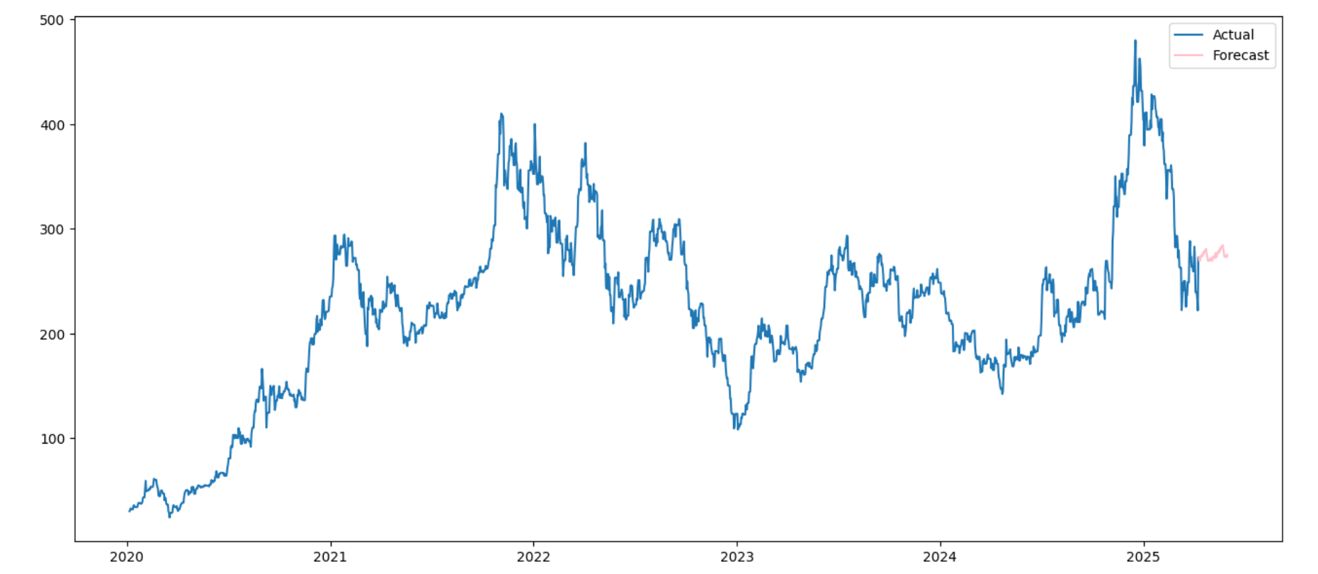
forecast = ARIMA_model_forecast(df,forecast_end_date)
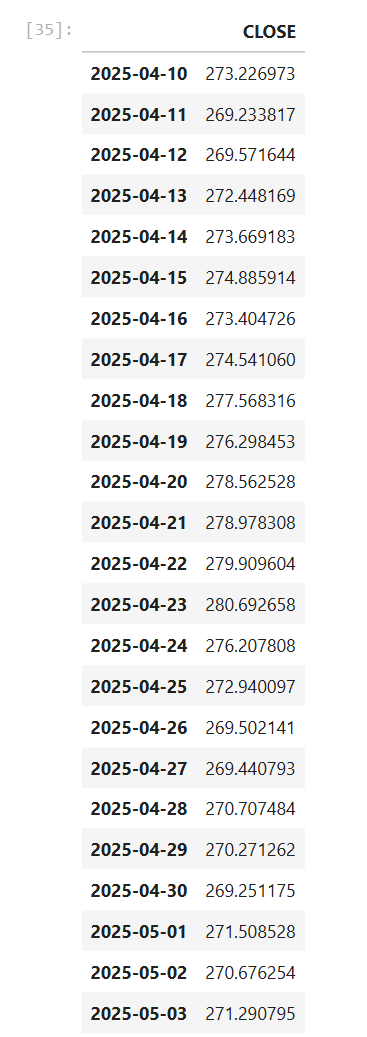
#display forecast time series
forecast

The code plots a graph consisting of the actual time series got from get_history() function and forecast time series using ARIMA model. Then, display the forecast time series like an example below:

That covers a code walkthrough.

Conclusion

At the end of this article, you should be able to get time series from LSEG Workspace platform using get_history() function in Data Library for Python. Then, you can use the time series with ARIMA model to make forecasts or use the time series for other purposes.