


Overview and Hypothesis
Natural gas is a physically traded commodity. Gas consumption and therefore the future price of gas can be described and understood through its “fundamental market drivers” such as volume of supply and weather.
Residential and commercial gas consumption is the amount of gas used by gas consumers connected to the local gas distribution networks as opposed to consumers connected directly to the high-pressure grid, such as power stations and big industrial facilities. Residential and commercial gas consumption forecasts are crucial to operational planning and gas pricing. The difference between sectors in the way they consume gas also determines which fundamental drivers you might want to observe to understand the future supply-demand picture and therefore the price. For instance, residential demand is highly coupled to temperature whereas gas-for-power demand is less coupled to weather but more price sensitive.
To observe any correlation that may exist we can combine in a chart RICs pricing data from the Eikon Data API and consumption actuals and forecasts via RDMS REST API. To demonstrate this, we will consider the largest gas demand Country in Europe, Germany, and compare it to Europe's most liquid future hub price, TTF. The German market actual consumption data is reported by Trading Hub Europe (THE) as two distinct sectors:
- SLP - Residential Local Distribution Zone consumption (LDZ),
- RLM - combination of Industrial and Gas-for-power Consumption (RLM).
Below we will plot the TTF Daily Close price RIC against actual consumption. We will also take this further by benchmarking several available forecasts from RDMS for gas consumption which are produced by the European Gas Team.
Prerequisites
- A Python environment with the Eikon Data API package installed.
- Every application using the Eikon Data API must identify itself with an Application Key or App Key for short. This Key, that is a unique identifier for your application, must be created using the App Key Generator application in Eikon Desktop/ LSEG Workspace that you can find in via the toolbar of Eikon/ Workspace. How to run it and create an App Key for a new application is available in the Eikon Data API Quick Start Guide and here's the Eikon Data API Overview page
- The list of Python package version can be found in the find requirements.txt in the GitHub code repository attached at the top right of this article
- RDMS account with a subscription to the European Gas Package.
- Refinitiv Data Management Solutions (RDMS), more detail can be found here. You will get an account to access the specific instance of RDMS that contains the data set that you're interested in. It's recommended to follow the RDMS REST API Quick Start Guide to do the User Setup, Registration, Manage your account, Access the RDMS Administrator Web Application, and Access the RDMS Swagger REST API Page.
The guide to generating the RDMS API key, which is required for accessing data via RDMS API, is also provided in the quick start guide.
- Refinitiv Data Management Solutions (RDMS), more detail can be found here. You will get an account to access the specific instance of RDMS that contains the data set that you're interested in. It's recommended to follow the RDMS REST API Quick Start Guide to do the User Setup, Registration, Manage your account, Access the RDMS Administrator Web Application, and Access the RDMS Swagger REST API Page.
- Generated API keys for both Eikon Data API and RDMS API to enable direct data feeds which are stored within a text file named api_key.txt on your computer in the format below.
Replace your valid keys on YOUR_EIKON_DATA_API_KEY and YOUR_RDMS_API_KEY
key,value
eikon_api_key,YOUR_EIKON_DATA_API_KEY
RDMS_api_key,YOUR_RDMS_API_KEY
Step-by-Step Guide to visualizing data
A full Jupyter notebook file with the codes, visualisation, comments, and guidance has been uploaded and can is accessible on the link in the top-right of this article.
Below is an example of how to connect to Eikon Data API and RDMS API to plot curve and RICS data together. This will enable the observation of any correlation between price and fundamental price driver.
- We access the TTF Daily close price from the Eikon Data API.
- We access EU Gas Actuals and Forecast data from RDMS.
At the end of this article, we will plot:
- Actual consumption
- The latest EC15 and EC46 forecasts
- A range of EC15 forecasts from the past year
- We will use the Meta data from RDMS to populate the graph automatically
- Plot DA close price to observe correlations.
Step 1 ) Preamble
In this step, we do the package import, API keys loading (from text file api_key.txt), set up connections for RDMS and Eikon Data API, and define the Curve IDs and RICs that we're interested.
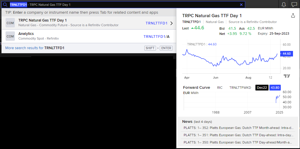
- The RIC used in this example is TRNLTTFD1, which is the daily close price of TTF Gas. Below is its information in the Workspace application.
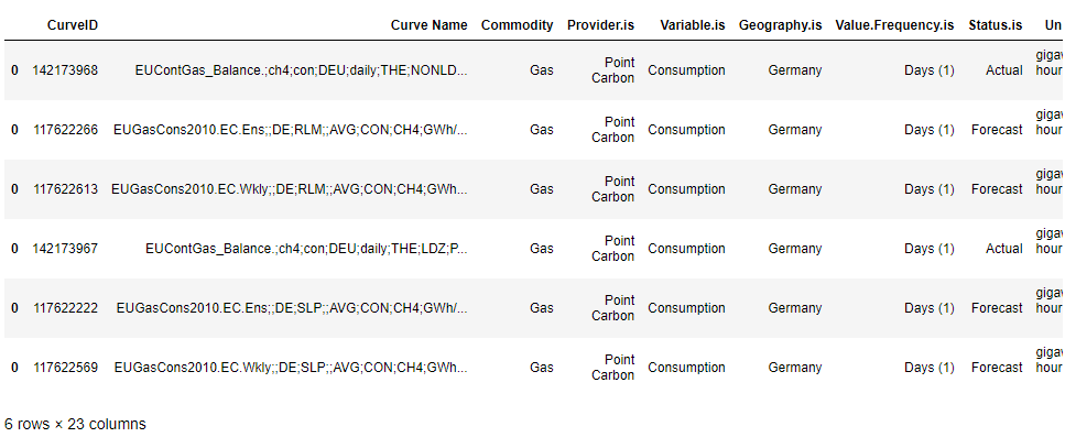
- Curve IDs used here are the German actuals and forecasts of Methane gas of industrial and residential below is their metadata printed out with the code in the notebook
- Two sets of curve ID are used, each three of them are the actual and forecast of Industrial Consumption (RLM) and residential Consumption (SLP).
- First we are going to plot for the SLP, so the RLM set is commented out
- To plot the RLM, uncomment the RLM set and comment the SLP set out instead
"""
# DE RLM
DE_actuals=142173968
DE_Forecast_EC15=117622266 # EC15, freq = hours
DE_Forecast_EC46=117622613 # EC46, freq = twice a week
"""
# DE SLP
DE_actuals=142173967
DE_Forecast_EC15=117622222 # EC15, freq = hours
DE_Forecast_EC46=117622569 # EC46, freq = twice a week
Step 2) Useful times and dates
Generate the start and end datetime that we are going to retrieve the forecast and actual value. To cover all the data needed, we go back 6 years and forwards to the end of next calendar year. For example, if this year is 2023, we're retrieving the data from year 2017 - 2024.
Today= datetime.today()
# Dates to pull data between
# To cover all the data needed we go back 6 years and forwards to end of next calander year.
Forecast_start = datetime(year=Today.year-6, month = 1, day = 1)
Forecast_end = datetime(year=Today.year+1, month = 12, day = 1)
# Value date range
Value_start = Forecast_start
Value_end = Forecast_end
print('Date range: from {} \n to {}'.format(Forecast_start, Forecast_end));
Step 3) My Functions
These four functions are written.
3.1 ) get_RDMS_meta: retrieves curve metadata from RDMS
def get_RDMS_meta(url,CurveID):
'''
This function retrives curve meta from RDMS
'''
CURVE=url+str(CurveID)
response = requests.request("GET",CURVE , headers=headers).content
rawData = pd.read_csv(io.StringIO(response.decode('utf-8')))
return rawData
3.2) get_RDMS_data: retrieves data from RDMS
def get_RDMS_data(url,CurveID,Value_start,Forecast_start=None):
'''
This function retrives data from RDMS
'''
if Forecast_start == None:
CURVE=url+str(CurveID)
MinValueDate=str(Value_start).replace(" ","T")
CURVE=CURVE+"?MinValueDate="+MinValueDate
else:
CURVE=url+str(CurveID)
MinValueDate=str(Value_start).replace(" ","T")
MinForecastDate=str(Forecast_start).replace(" ","T")
CURVE=CURVE+"?MinForecastDate="+MinForecastDate+"&MinValueDate="+MinValueDate
print (CurveID,"->", CURVE)
response = requests.request("GET",CURVE , headers=headers).content
rawData = pd.read_csv(io.StringIO(response.decode('utf-8')))
return rawData
3.3) sort_forecast: produces dictonary of forecast data using the datetime stamp as a key to allows easy plotting of various forecasts
def sort_forecast(dataF):
'''
This produces dictonary of forecast data using the datetime stamp as KEY.
Allows for easy plotting of various forecasts
'''
Forecasts={}
Forecast_FD=dataF.groupby("ForecastDate")
for G in Forecast_FD:
# clean up key for nice visual
KEY=str(G[0]).replace("Timestamp","").replace("'","")
Forecasts[KEY]=G[1].drop(columns=["ForecastDate"]).set_index("ValueDate").rename({"Value":KEY},axis=1)
# Clean up naming from UTC back to CET
for K in list(Forecasts.keys()):
new_key=K.replace('01:00:00','00:00:00').replace('02:00:00','00:00:00').replace('13:00:00','12:00:00').replace('14:00:00','12:00:00')
Forecasts[new_key] = Forecasts.pop(K)
Forecasts[new_key].rename({K:new_key},axis=1,inplace=True)
return Forecasts
3.4) create_daily_forecast: creates a daily forecast from either EC15 or EC46 data i.e. Day ahead forecast is day Which_forecast_day= 1
def create_daily_forecast(EC,Which_forecast_day,Forecasts):
'''
This creates a daily forecast from either EC15 or EC46 data.
ie Day ahead forecast is day Which_forecast_day= 1
'''
daily_forecast=pd.DataFrame(columns=["DA-"+str(Which_forecast_day)+" Forecast","ForecastDate"])
for i, fil in enumerate(list(Forecasts.keys())):
if EC+":" in fil:
DAV=Forecasts[fil].iloc[Which_forecast_day].values[0]
daily_forecast.loc[i,"DA-"+str(Which_forecast_day)+" Forecast"]=DAV
daily_forecast.loc[i,"ForecastDate"]=fil.split(" ")[0]
daily_forecast=daily_forecast.set_index("ForecastDate")
daily_forecast.index=daily_forecast.index.astype('datetime64[ns]')
return daily_forecast
Step 4) Curves and metadata
Extract the metadata to be used in the graph decoration
Meta_actuals=get_RDMS_meta(url_meta,DE_actuals).T.rename({0:"meta"},axis=1).rename({"":"Meta"},axis=1)
# For use in the graph decoration
Sector = Meta_actuals.loc["Sector.is"][0]
Country = Meta_actuals.loc["Geography.is"][0]
Unit = Meta_actuals.loc["Unit"][0]
Variable = Meta_actuals.loc["Variable.is"][0]
print(Meta_actuals.index)
Step 5) Get RDMS data and format them
5.1 ) Get actuals and forcast data from RDMS
# Get actuals data
dataA=get_RDMS_data(url,DE_actuals,Value_start,None)
dataA=dataA.drop(columns=["ForecastDate","ScenarioID"]) # Drop forecast date as this is a time series curve
dataA["ValueDate"]= pd.to_datetime(dataA["ValueDate"])
dataA=dataA.rename({"Value":"Actuals"},axis=1).set_index("ValueDate") # Rename and set index
# Forecast data for EC15.
dataF_EC15=get_RDMS_data(url,DE_Forecast_EC15,Value_start,Forecast_start)
dataF_EC15=dataF_EC15.drop(columns=["ScenarioID"])
dataF_EC15["ValueDate"]= pd.to_datetime(dataF_EC15["ValueDate"])
# Forecast data for EC46.
dataF_EC46=get_RDMS_data(url,DE_Forecast_EC46,Value_start,Forecast_start)
dataF_EC46=dataF_EC46.drop(columns=["ScenarioID"])
dataF_EC46["ValueDate"]= pd.to_datetime(dataF_EC46["ValueDate"])
Below are the endpoints with parameters
142173967 -> https://analyst.rdms.refinitiv.com/api/v1/CurveValues/142173967?MinValueDate=2017-01-01T00:00:00
117622222 -> https://analyst.rdms.refinitiv.com/api/v1/CurveValues/117622222?MinForecastDate=2017-01-01T00:00:00&MinValueDate=2017-01-01T00:00:00
117622569 -> https://analyst.rdms.refinitiv.com/api/v1/CurveValues/117622569?MinForecastDate=2017-01-01T00:00:00&MinValueDate=2017-01-01T00:00:00
5.2) Sort forecasts in dict and convert to UTC
Forecasts_EC15=sort_forecast(dataF_EC15)
Forecasts_EC46=sort_forecast(dataF_EC46)
5.3) Create a day ahead of forecast
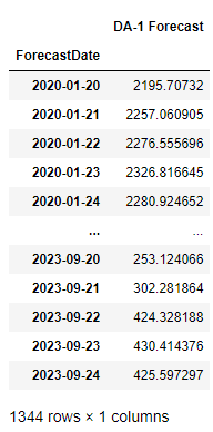
If we take the first day of each forecast, this will be the Day Ahead forecast which will be the most predictive forecast in terms of weather forecast error impact predicability. We can do this for any of our forecasts (EC,GFS, ENS or Op). Here, we use our EC12 forecast which used for our morning comment.
EC="12"
Which_forecast_day=1 # EC12 - 1 to 15 days out possible
Day_ahead=create_daily_forecast(EC,Which_forecast_day,Forecasts_EC15)
Day_ahead
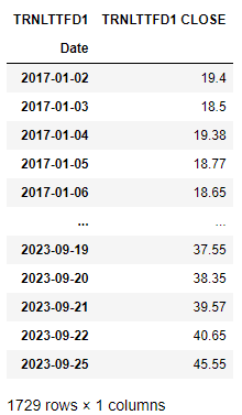
Step 6) Get prices
Use get_timeseries function in Eikon Data API to get the close prices of the instrument defined
PRICES=ek.get_timeseries(rics,fields='CLOSE',start_date=Forecast_start.strftime('%Y-%m-%d'))
PRICES=PRICES.rename({PRICES.columns[0]:str(rics[0])+" "+PRICES.columns[0]},axis=1) #Rename to at price type into name
PRICES
Step 7) Plot actuals and forecast
Using the interactive notebook plots with Matplotlib widget, we do the graph plotting from the data we have retrieved.
You can check the full Jupyter notebook file with the codes, visualisation, comments, and guidance with the link in the top-right of this article.
Observations and Conclusions
Using the notebook, we were able to easily plot data using a matplotlib a chart to compare TTF price, actual consumption data and forecast consumption data. Two graphs can be seen in Figures 1 and 2 respectively. Firstly, SLP plotted against TTF and secondly RLM plotted against TTF.

Figure 1 – German SLP demand actuals benchmarked against weather based, EC15, EC46 and Day Ahead forecasts. TTF Daily Close price is also plotted on a second axis.
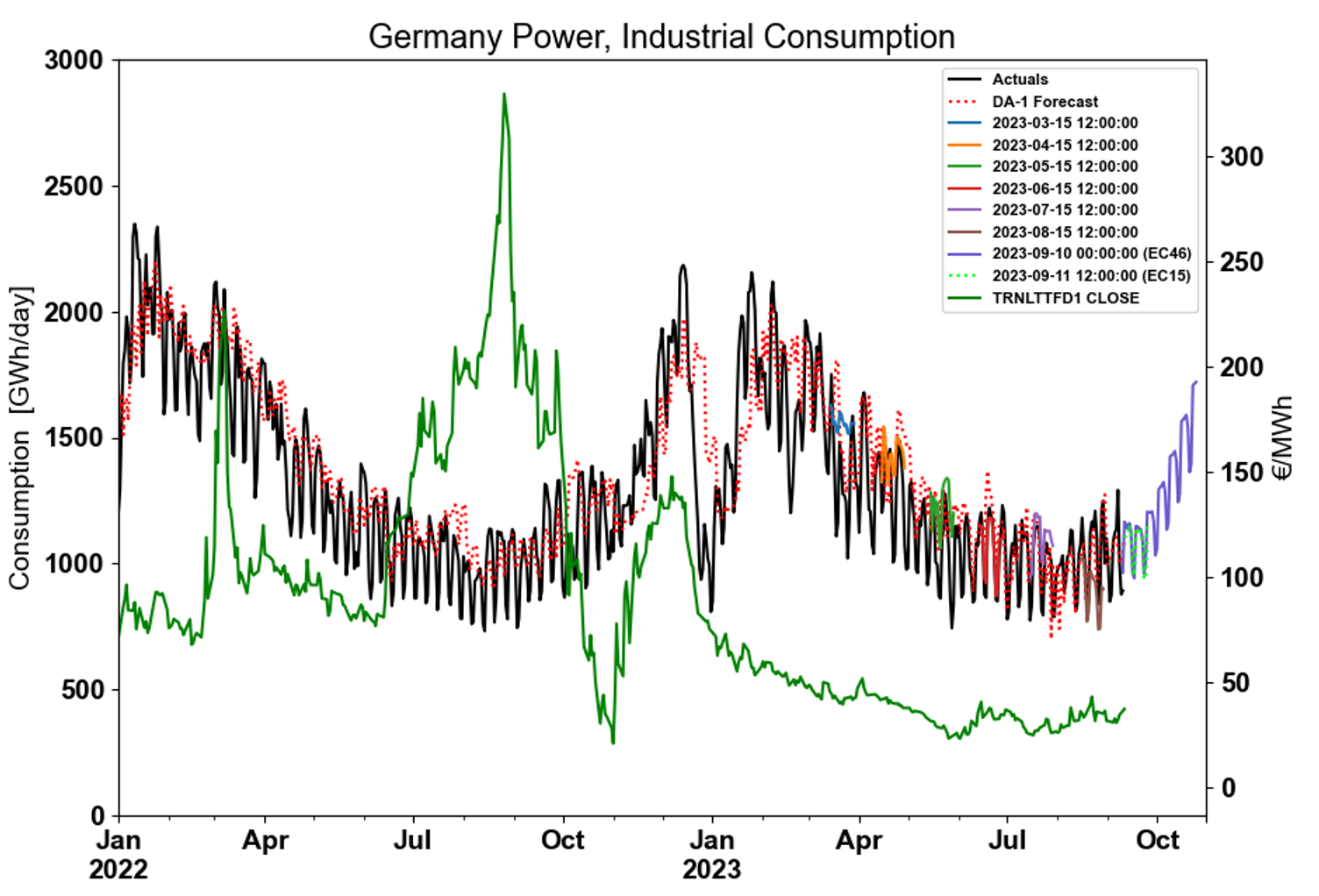
Figure 2– German RLM demand actuals benchmarked against weather-based forecasts and plotted with TTF Daily Close price.
- Both the EC15 and EC46 forecasts correlate well with historical actuals consumption data.
- SLP and RLM have different consumption profiles.
- SLP is seasonal, temperature driven and increases significantly in winter.
- RLM demand has an added weekly periodicity to its profile due to demand being lower at weekends.
- There are clear times of the year such as at the start of the calendar year where the drop in consumption correlates to a general fall in TTF price for both SLP and RLM.
- TTF price in summer 2022 was primarily driven by supply-side concerns and influenced heavily by sentiment-based volatility. This meant prices decoupled from fundamental drivers and prices spiked. This is clear when comparing this to 2023 which saw a more “typical” price profile for TTF which is decreasing in summer as European Storages get filled.
References
- EU RESIDENTIAL & COMMERCIAL GAS CONSUMPTION MODEL Methodology paper on Workspace
- Trading Hub Europe: https://www.tradinghub.eu/
For any questions related to the RDMS and Eikon Data API usage, feel free to visit or ask you question in the Developers Community Q&A Forum.
- Register or Log in to applaud this article
- Let the author know how much this article helped you