


Introduction to 3D Investing
Traditional mean-variance portfolio optimization often considers only 2 investing objectives which are risk and return (2D). 3D investing, on the other hand, adds sustainability as an additional objective to optimize risk and return, as well as sustainability objectives.
adding the sustainability metric in the objective function (using a multi-objective optimization framework)
The classic mean-variance optimization problem can be written as:
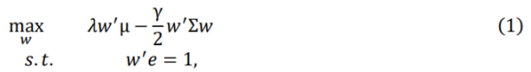
where 𝑤 is an 𝑁 × 1 vector of asset weights, 𝜇 is an 𝑁 × 1 vector of expected returns, Σ is the 𝑁 × 𝑁 variance-covariance matrix, 𝑒 is an 𝑁 × 1 vector of ones, and 𝜆 and 𝛾 are scalar coefficients.
Portfolios generated under Eq. (1) are mean-variance optimal in that they achieve the maximum expected return for a given level of risk.” – 3D Investing: Jointly Optimizing Return, Risk, and Sustainability
The traditional approach of standard mean-variance optimization can readily be extended to mean variance-sustainability optimization by applying sustainability factors alongside traditional risk and return considerations.
It is straightforward to extend the mean-variance optimizer from Eq. (1) to construct portfolios on an efficient frontier surface in three (or more) dimensions. In the case of additional sustainability considerations, Eq. (1) can be extended to three dimensions as follows:
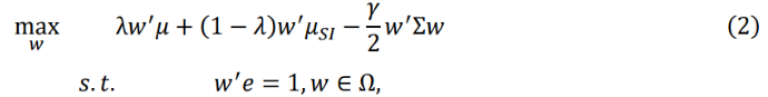
where 𝜇𝑆𝐼 is an 𝑁 × 1 vector of any (discrete or continuous) sustainability metric, 𝜆 becomes the relative preference between the return and sustainability objectives, and Ω is the set of feasible solutions, which includes any portfolio constraints.” – 3D Investing: Jointly Optimizing Return, Risk, and Sustainability
Studies suggest 3D investing can achieve better results than traditional methods, especially for portfolios with ambitious sustainability goals.
Prerequisites
- LSEG Workspace application with an access for RD library desktop session.
- Python 3.9 or above
- Python libraries
- pandas==2.1.4
- numpy==1.25.0
- refinitiv-data==1.6.0
- scipy==1.9.3
- matplotlib==3.8.0
- matplotlib-inline==0.1.6
- plotly==5.22.0
Python Code Implementation
First we're importing necessary libraries and open the data library session (some other libraries such as scipy, matplotlib, plotly will be imported in the step of visualization and analysis)
import pandas as pd
import numpy as np
import refinitiv.data as rd
rd.open_session()
# Define list of RICs for the interested instrument
rics = ['SCC.BK','PTT.BK','ADVANC.BK']
Step 1) Prepare datasets for factor modeling.
In this demonstration utilized two datasets – asset price dataset and ESG scoring dataset. The asset price dataset contains the daily closing price of the asset. The ESG score dataset contains the ESG score across multiple domains of the corresponding asset. In this demonstration, we select 3 different assets for the portfolio.
We're using a list of RICs SCC.BK, PTT.BK, ADVANC.BK here, it can be changed to the instrument you're interested or chain, such as 0#.SETI for SET Index
The RIC (Refinitiv Identification Code) is a market-level identifier for instruments and pricing sources. To find the RIC you're looking for, you can use
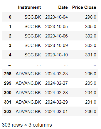
Price Data
# Get pricing data with get_data function
price_df = rd.get_data(rics,
['TR.PriceClose.date', 'TR.PriceClose'],
{'SDate': '2023-10-04', 'EDate': '2024-03-01', 'Frq': 'D'})
price_df['Price Close'] = price_df['Price Close'].astype(int)
price_df
ESG Score Data
# Get ESG score data with get_data function
esg_df = rd.get_data(
universe = rics,
fields = [
'TR.TRESGScore.date',
'TR.TRESGScore',
'TR.TRESGCScore',
'TR.TRESGCControversiesScore',
'TR.TRESGResourceUseScore',
'TR.TRESGEmissionsScore',
'TR.TRESGInnovationScore',
'TR.TRESGWorkforceScore',
'TR.TRESGHumanRightsScore',
'TR.TRESGCommunityScore',
'TR.TRESGProductResponsibilityScore',
'TR.TRESGManagementScore',
'TR.TRESGShareholdersScore',
'TR.TRESGCSRStrategyScore'
]
)
esg_df
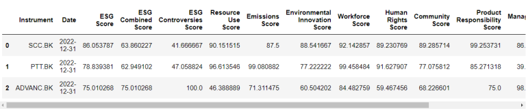
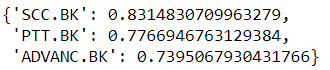
2) Calculate ESG Score of Each Asset
LSEG has developed an ESG scoring framework, aimed at providing a transparent and objective measure of a company’s ESG performance. Here we're using the ESG score on the latest date to calculate the mean ESG score of each asset.
# Calculate mean ESG score of each asset
asset_esg = {}
for i in range (3):
asset_esg[esg_df['Instrument'][i]] = esg_df.iloc[i, 2:-2].mean() * 0.01
asset_esg
Mean ESG score of each asset is as below
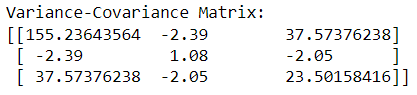
3) Calculate Variance-Covariance Matrix
Calculate variance-covariance matrix from closing price of each dataset
asset_returns = {}
for ric in rics:
# Historical returns of 3 assets over time
asset_returns[ric] = np.array(price_df[price_df['Instrument']== ric]['Price Close'])
returns_matrix = np.vstack((asset_returns['SCC.BK'], asset_returns['PTT.BK'], asset_returns['ADVANC.BK']))
# Calculate the variance-covariance matrix
covariance_matrix = np.cov(returns_matrix)
print("Variance-Covariance Matrix:")
print(covariance_matrix)
Here's the result
4) 3D Optimization
Initializing variables and defining objective function and sustainability constraints, the optimized portfolio weights of each asset can be calculated
from scipy.optimize import minimize
# Expected returns for 3 securities
expected_returns = np.array([0.10, 0.12, 0.11])
# Variance-covariance matrix
risk_matrix = covariance_matrix
# Sustainability scores for each security
sustainability_scores = np.array([asset_esg['SCC.BK'], asset_esg['PTT.BK'], asset_esg['ADVANC.BK']])
# Current portfolio weights
current_weights = np.array([0.2, 0.2, 0])
# Coefficient for returns
λ1 = 0.5
# Coefficient for sustainability
λ2 = 0.5
# Risk aversion coefficient
γ = 0.1
# Objective function
def objective(weights):
returns = np.dot(weights, expected_returns)
sustainability = np.dot(weights, sustainability_scores)
risk = np.dot(weights.T, np.dot(risk_matrix, weights))
turnover_penalty = np.sum((weights - current_weights)**2)
return -(λ1 * returns + λ2 * sustainability - γ/2 * risk - turnover_penalty)
# Constraints
def sustainability_constraint(weights):
return np.dot(weights, sustainability_scores) - minimum_sustainability_score
# Minimum desired sustainability score for the portfolio
minimum_sustainability_score = 0.75
cons = [{'type': 'eq', 'fun': lambda x: np.sum(x) - 1}, # Sum of weights must be 1
{'type': 'ineq', 'fun': sustainability_constraint}] # Portfolio sustainability score constraint
# Weights must be between 0 and 1
bounds = [(0, 1) for _ in range(len(expected_returns))]
# Optimization
result = minimize(objective,
current_weights,
method='SLSQP',
bounds=bounds,
constraints=cons)
# Optimized weights
optimized_weights = result.x
print("Optimized Portfolio Weights:", optimized_weights)
And the result is

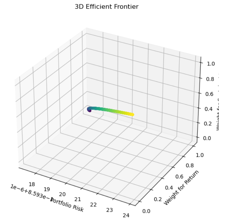
3D Efficient Frontier
Visualizes the 3D efficient frontier of a portfolio optimization considering returns, risk, and sustainability. We do two visualizations here as below
- First visualization
import matplotlib.pyplot as plt
# Number of portfolios to simulate on the efficient frontier
num_portfolios = 1000
# Store results
results = np.zeros((4, num_portfolios))
for i in range(num_portfolios):
# Adjusting the weights for the objectives (return, risk, sustainability)
λ1 = i / (num_portfolios - 1) # Weight for return
λ2 = 1 - λ1 # Weight for sustainability
# Objective function for optimization
def objective(weights):
returns = np.dot(weights, expected_returns)
risk = np.dot(weights.T, np.dot(risk_matrix, weights))
sustainability = np.dot(weights, sustainability_scores)
return -(λ1 * returns + λ2 * sustainability - risk)
# Constraints
def sustainability_constraint(weights):
return np.dot(weights, sustainability_scores) - minimum_sustainability_score
minimum_sustainability_score = 0.75 # Minimum desired sustainability score for the portfolio
cons = [{'type': 'eq', 'fun': lambda x: np.sum(x) - 1}, # Sum of weights must be 1
{'type': 'ineq', 'fun': sustainability_constraint}] # Portfolio sustainability score constraint
bounds = [(0, 1) for _ in range(len(expected_returns))] # Weights must be between 0 and 1
# Perform optimization
initial_guess = np.array([1 / len(expected_returns)] * len(expected_returns))
result = minimize(objective, initial_guess, method='SLSQP', bounds=bounds, constraints=cons)
# Store results
results[0, i] = λ1 # Weight for return
results[1, i] = λ2 # Weight for sustainability
results[2, i] = -result.fun # Portfolio objective value
results[3, i] = np.sqrt(np.dot(result.x.T, np.dot(risk_matrix, result.x))) # Portfolio risk (standard deviation)
# Plotting the 3D efficient frontier
fig = plt.figure(figsize=(10, 7))
ax = fig.add_subplot(111, projection='3d')
ax.scatter(results[3, :], results[0, :], results[1, :], c=results[1, :], cmap='viridis')
ax.set_xlabel('Portfolio Risk')
ax.set_ylabel('Weight for Return')
ax.set_zlabel('Weight for Sustainability')
ax.set_title('3D Efficient Frontier')
plt.show()
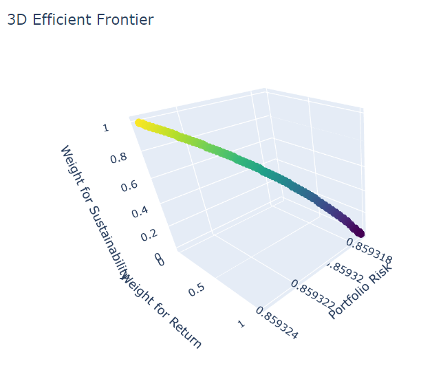
- Second visualization
import plotly.graph_objects as go
# Creating a Plotly figure
fig = go.Figure(data=[go.Scatter3d(
x=results[3, :],
y=results[0, :],
z=results[1, :],
mode='markers',
marker=dict(
size=5,
color=results[2, :], # set color to objective value
colorscale='Viridis', # choose a colorscale
opacity=0.8
)
)])
# Adding labels and title
fig.update_layout(
scene=dict(
xaxis_title='Portfolio Risk',
yaxis_title='Weight for Return',
zaxis_title='Weight for Sustainability'
),
title='3D Efficient Frontier'
)
# Show the plot
fig.show()
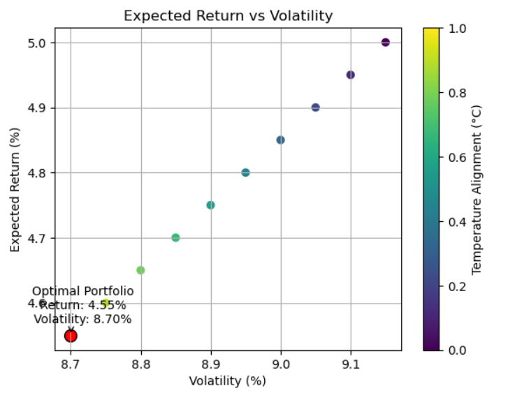
Lastly, let's plot the graph to see the relation between Expected Return and Volatility
import matplotlib.pyplot as plt
# Assuming the following data structure
# Portfolios data: Each portfolio has expected return, volatility, and temperature alignment
portfolios_data = np.array([
[4.30, 8.45, 2.6], [4.35, 8.50, 2.55], [4.40, 8.55, 2.50],
[4.45, 8.60, 2.45], [4.50, 8.65, 2.40], [4.55, 8.70, 2.35],
[4.60, 8.75, 2.30], [4.65, 8.80, 2.25], [4.70, 8.85, 2.20],
[4.75, 8.90, 2.15], [4.80, 8.95, 2.10], [4.85, 9.00, 2.05],
[4.90, 9.05, 2.00], [4.95, 9.10, 1.95], [5.00, 9.15, 1.90]
])
# Filter portfolios by a temperature target, e.g., 2.35°C
temperature_target = 2.35
portfolios = portfolios_data[portfolios_data[:, 2] <= temperature_target]
# Risk aversion scenarios (low, medium, high)
risk_aversions = ['low', 'medium', 'high']
risk_aversion_weights = {
'low': 0.1,
'medium': 0.5,
'high': 0.9
}
# Select medium risk aversion
selected_risk_aversion = 'medium'
# Calculate the optimal portfolio based on the selected risk aversion
# The optimal portfolio minimizes volatility given the expected return
weights = risk_aversion_weights[selected_risk_aversion]
optimal_portfolio = min(portfolios, key=lambda x: weights * x[1] - (1 - weights) * x[0])
# Create scatter plot for expected return vs volatility
plt.scatter(portfolios[:, 1], portfolios[:, 0], c=portfolios[:, 2], cmap='viridis')
# Highlight the optimal portfolio
plt.scatter(optimal_portfolio[1], optimal_portfolio[0], color='red', edgecolors='black', s=100)
# Annotate the optimal portfolio
plt.annotate(
f"Optimal Portfolio\nReturn: {optimal_portfolio[0]:.2f}%\nVolatility: {optimal_portfolio[1]:.2f}%",
(optimal_portfolio[1], optimal_portfolio[0]),
textcoords="offset points",
xytext=(10,10),
ha='center',
arrowprops=dict(arrowstyle="->", connectionstyle="arc3,rad=.2")
)
# Set chart title and labels
plt.colorbar(label='Temperature Alignment (°C)')
plt.title('Expected Return vs Volatility')
plt.xlabel('Volatility (%)')
plt.ylabel('Expected Return (%)')
plt.grid(True)
# Show the plot
plt.show()
Conclusion
The 3D framework is a valuable tool for investors seeking to integrate sustainability into their portfolio construction while maintaining financial objectives. By utilizing the 3D investing framework, investors can construct portfolios that meet specific sustainability targets (e.g., carbon footprint reduction) without sacrificing returns or incurring excessive costs.
- Register or Log in to applaud this article
- Let the author know how much this article helped you