


Introduction to ESG
In recent years, sustainability in business has been brought to attention, and there has been a growing recognition among investors about the importance of Environmental, Social, and Governance (ESG) factors in investment analysis. These factors are seen as integral to evaluating a company's long-term sustainability and risk profile. Many investors seek to align their portfolios with their sustainability values, and this has led to the rise of ESG investing.
ESG is a framework for evaluating a company's performance and impact considering three main area:
- Environmental: Assessing a company's impact on the environment, including its carbon footprint, pollution levels, and resource management practices.
- Social: Examining a company's relationships with its stakeholders, including employees, customers, and communities. This could involve factors like labor practices, diversity and inclusion, and community engagement.
- Governance: Focusing on a company's leadership structure, transparency, accountability, and risk management practices. Strong governance helps ensure long-term sustainability and mitigates risks like fraud or mismanagement.
London Stock Exchange Group (LSEG) has developed our own ESG scoring framework, aimed at providing a transparent and objective measure of a company’s ESG performance. This framework evaluates companies based on their relative performance, commitment, and effectiveness across 10 main themes, encompassing a wide range of criteria from environmental sustainability to corporate governance and social responsibility
Factor Modeling
Factor modeling seeks to explain the returns of a stock or portfolio by attributing them to various factors, each representing a specific characteristic or attribute that influences stock prices. Factor models are typically constructed using historical data through techniques such as regression analysis. Integration of ESG scores with factor models can be done by treating them as additional factors. This allows investors to incorporate sustainability considerations into their investment strategies.
Prerequisites
- LSEG Workspace application with an access for RD library desktop session.
- Python 3.9 or above
- Python libraries
- pandas==2.1.4
- numpy==1.25.0
- seaborn==0.13.2
- matplotlib==3.8.0
- matplotlib-inline==0.1.6
- refinitiv-data==1.6.0
- scikit-learn==1.4.2
- scipy==1.9.3
Python Code Implementation
First we're importing necessary libraries and open the data library session (some other libraries such as scipy and sklearn will be imported in the step of visualization and analysis)
import pandas as pd
import numpy as np
import seaborn as sns
import matplotlib.pyplot as plt
import refinitiv.data as rd
rd.open_session()
Step 1) Prepare datasets for factor modeling.
In this demonstration utilized two datasets – asset price dataset and ESG scoring dataset. As the ESG score data is available in annually interval, our asset price dataset also contains the annually closing price of the asset. The ESG score dataset contains the ESG score across multiple domains of the corresponding asset, which will be used as factors in this modeling.
We're using RIC SCC.BK here, it can be changed to the instrument you're interested or chain, such as 0#.SETI for SET Index
The RIC (Refinitiv Identification Code) is a market-level identifier for instruments and pricing sources. To find the RIC you're looking for, you can use
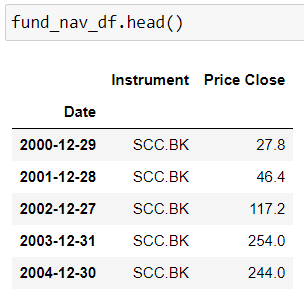
# Get annual pricing data with get_data function from year 2000 to 2024
fund_nav_df = rd.get_data(['SCC.BK'],
['TR.PriceClose.date', 'TR.PriceClose'],
{'SDate': '2000-10-04', 'EDate': '2024-03-01', 'Frq': 'FY'})
fund_nav_df.set_index('Date', inplace=True)
fund_nav_df
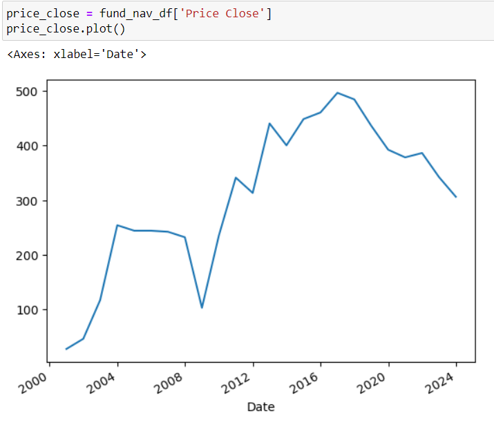
# Plot graph to see the trend of pricing
price_close = fund_nav_df['Price Close']
price_close.plot()
Prepare ESG score data
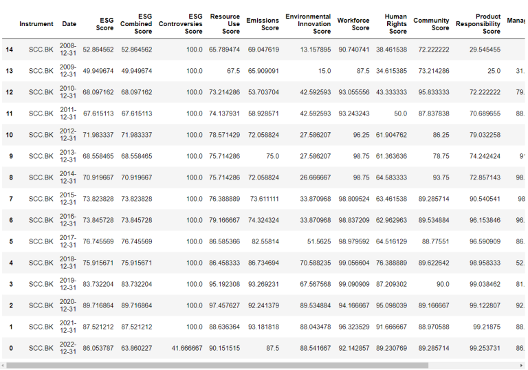
# Get annual ESG score data with get_data function from year 2000 to 2024
df = rd.get_data(
universe = ['SCC.BK'],
fields = [
'TR.TRESGScore.date',
'TR.TRESGScore',
'TR.TRESGCScore',
'TR.TRESGCControversiesScore',
'TR.TRESGResourceUseScore',
'TR.TRESGEmissionsScore',
'TR.TRESGInnovationScore',
'TR.TRESGWorkforceScore',
'TR.TRESGHumanRightsScore',
'TR.TRESGCommunityScore',
'TR.TRESGProductResponsibilityScore',
'TR.TRESGManagementScore',
'TR.TRESGShareholdersScore',
'TR.TRESGCSRStrategyScore'
],
parameters = {'Period':'FY0','Frq':'FY','SDate':'0','EDate':'-24'}
)
# Format data
factor_df = df
factor_df.sort_values(by = ['Date'], ascending = [True], inplace = True)
factor_df.dropna(inplace=True)
factor_df
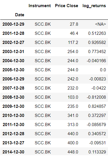
Step 2) Calculate Log Return of asset
Calculate annually log returns from asset price dataset to observe price behavior, which will serve as the dependent variable in regression analysis.
# Calculate Log Return of Asset
log_returns = np.log(price_close / price_close.shift(1))
fund_nav_df["log_returns"] = log_returns
fund_nav_df
Step 3) Merge Datasets and Map ESG Scores
Merge datasets by years into a single dataframe and map ESG scores to corresponding assets.
fund_nav_df.drop(columns=['Instrument', 'Price Close'], inplace = True)
fund_nav_df['Year'] = fund_nav_df.index.strftime('%Y')
factor_df['Year'] = factor_df['Date'].dt.strftime('%Y')
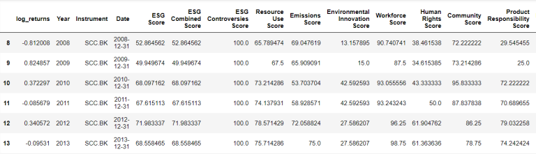
df_beta = pd.merge(fund_nav_df, factor_df , on='Year', how='left').dropna()
df_beta
Step 4) Linear Regression
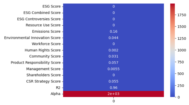
Performing linear regression on the entire dataset to assess the relationship between log returns and ESG factors. Log return data are assigned to y value and all corresponding factors are assigned as X value. Calculate R-Squared and regression intercept (Alpha) values.
from sklearn.linear_model import LinearRegression
from sklearn.metrics import r2_score
# Log return data are assigned to y value
y = df_beta.iloc[:, 1:2].to_numpy()
# All corresponding factors are assigned as X value
X = df_beta.drop(columns=['log_returns','Year','Instrument','Date'])
# coefficients linear regression
reg = LinearRegression(positive = True).fit(X, y)
liber_coeff = pd.DataFrame(reg.coef_, columns=reg.feature_names_in_)
# Calculate R-Squared and regression intercept (Alpha) values
R2 = r2_score( y, reg.predict(X))
liber_coeff["R2"] = R2
liber_coeff["Alpha"]=reg.intercept_
liber_coeff
Then we plot it as a heatmap graph as below
sns.heatmap(liber_coeff.T, annot=True, cmap='coolwarm')
plt.show()
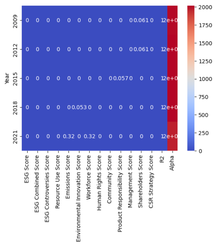
To capture any relationship between different time periods within the dataset, performing linear regression on a subset of the dataset. Identifying variations in the relationship between variables across subsets.
# Performing linear regression on a subset of the dataset
# Identifying variations in the relationship between variables across subsets.
list_factor_year = []
x = range(0, len(df_beta), 3)
for n in x:
df_beta_ = df_beta.iloc[n:n+2].drop(columns=['Date'])
y = df_beta_.iloc[:, 1:2].to_numpy()
X = df_beta_.drop(columns=['log_returns','Year','Instrument'])
# Coefficients linear regression
reg = LinearRegression(positive = True).fit(X, y)
liber_coeff = pd.DataFrame(reg.coef_, columns=reg.feature_names_in_)
R2 = r2_score(y, reg.predict(X))
liber_coeff['R2'] = R2
liber_coeff['Alpha']=reg.intercept_
liber_coeff['Year'] = df_beta_.Year.iloc[-1]
list_factor_year.append(liber_coeff)
df_factor_time = pd.concat(list_factor_year)
df_factor_time.set_index('Year', inplace=True)
df_factor_time
Then we plot it as a heatmap graph as below
sns.heatmap(df_factor_time.head(10), annot=True, cmap='coolwarm')
plt.show()
Step 5) Style Analysis
Find the optimal weights that minimizes the Tracking error between a portfolio of the explanatory variables(X) and the dependent variable(y). First, defining the styles_analysis function, then assigning asset log return (y value) as dependent variable and ESG factors (X value) as explanatory variables.
# Find the optimal weights that minimizes the Tracking error
# between a portfolio of the explanatory variables(X) and the dependent variable(y).
from scipy.optimize import minimize
def tracking_error(r_a, r_b):
"""
Returns the Tracking Error between the two return series
"""
return np.sqrt(((r_a - r_b)**2).sum())
def portfolio_tracking_error(weights, ref_r, bb_r):
"""
returns the tracking error between the reference returns
and a portfolio of building block returns held with given weights
"""
return tracking_error(ref_r, (weights*bb_r).sum(axis=1))
# Defining the styles_analysis function
def style_analysis(dependent_variable, explanatory_variables):
"""
Returns the optimal weights that minimizes the Tracking error between
a portfolio of the explanatory variables and the dependent variable
"""
n = explanatory_variables.shape[1]
init_guess = np.repeat(1/n, n)
bounds = ((0.0, 1.0),) * n # an N-tuple of 2-tuples!
# construct the constraints
weights_sum_to_1 = {'type': 'eq',
'fun': lambda weights: np.sum(weights) - 1
}
solution = minimize(portfolio_tracking_error, init_guess,
args=(dependent_variable, explanatory_variables,), method='SLSQP',
options={'disp': False},
constraints=(weights_sum_to_1,),
bounds=bounds)
weights = pd.Series(solution.x, index=explanatory_variables.columns)
return weights
# Assigning asset log return (y value) as dependent variable and ESG factors (X value) as explanatory variables
dependent_variable = df_beta[['log_returns']]
explanatory_variables = df_beta.iloc[:, 4:-1]
# Find the optimal weights that minimizes the Tracking error
weights_b = style_analysis(dependent_variable['log_returns'], explanatory_variables)
Then we plot it as a bar chart as below
weights_b.sort_values(ascending=False).plot.bar()
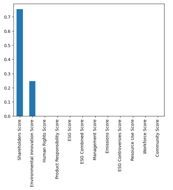
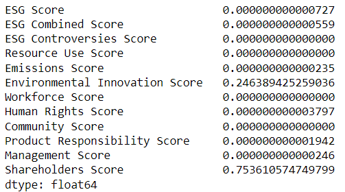
Here's the weights used to plot the chart above
pd.set_option('display.float_format', lambda x: '%.15f' % x)
weights_b
Conclusion
In conclusion, the integration of Environmental, Social, and Governance (ESG) factors into factor modeling represents a significant advancement in investment analysis. ESG considerations have become increasingly essential for investors seeking to align their portfolios with sustainability values while managing risk effectively.
Reference
- Register or Log in to applaud this article
- Let the author know how much this article helped you