

Raksina Samasiri
Developer Advocate
Developer Advocate
Introduction
Gold is not only a popular investment asset — it is also an important indicator of market uncertainty. When investors worry about global risks, they often buy gold, causing prices to move more sharply. Understanding volatility (how fast and how far the price moves) is essential for:
- Traders
- Analysts
- Risk managers
- Portfolio managers
- Anyone studying financial markets
In this tutorial, we will measure gold volatility in three different ways:
- Historical Volatility (HV) – based on past price movements
- Implied Volatility (IV) – based on option prices
- Volatility Smile – IV values across different deltas
Each method provides a different perspective:
| Type | Tells You |
|---|---|
| Historical Vol (HV) | What has already happened |
| Implied Vol (IV) | What traders expect to happen |
| Smile (Put & Call deltas) | Whether the market fears downside or upside more |
The LSEG Data Library allows us to retrieve all this data easily.
What Is Delta?
In options markets, delta tells you how sensitive an option is to the underlying price.
But for volatility, delta also tells you how far “out-of-the-money” an option is.
Think of delta like a temperature scale:
- 10‑delta = extreme
- 25‑delta = moderate
- 45‑delta = mild
- ATM vol (XAU3MO=R) ≈ 50‑delta = center point
Interpretation:
- Low delta puts → market fear of gold falling
- Low delta calls → market demand for upside spikes
- ATM delta → closest to current price (benchmark volatility)
Using many deltas helps build the volatility smile, which shows how volatility changes across different market scenarios.
Requirements
To follow along this article, you will need:
- LSEG Workspace running and logged-in on the same machine that uses to run Python script (To connect to the data platform with Desktop session, or a Platform Session license)
- Python 3 environment
- lseg-data Python library installed
- Basic understanding of Python and DataFrame operations
More detail can be found in the Quick Start guide.
Step-by-Step Guide to Retrieve the Data from the Data Library
Let's walk through each step with the explanation of its purpose.
Preparation step
Import necessary libraries, open the data library session to connect to the data platform, and declare start and end dates variables to be used in the request.
# Preparation step
import lseg.data as ld
from datetime import date, timedelta
import pandas as pd
import plotly.graph_objects as go
ld.open_session()
start = (date.today() - timedelta(days=730)).strftime('%Y-%m-%d')
end = date.today().strftime('%Y-%m-%d')
print(f'Start date: {start}, End date: {end}')
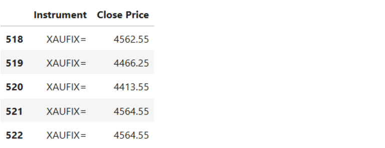
Step 1) Retrieve Gold Fixing Prices (XAUFIX=)
We start by loading gold fixing prices (similar to a daily benchmark). These prices are stable, widely available, and perfect for volatility calculations.
As we need a clean historical price series to compute Historical Volatility (HV) and the gold fixing (XAUFIX=) is the most consistent dataset across environments.
# Step 1) Retrieve Gold Fixing Prices (XAUFIX=)
gold = ld.get_data(
universe=['XAUFIX='],
fields=['TR.ClosePrice'], # Closing price
parameters={'SDate': start,
'EDate': end,
'Frq': 'D'}
)
display(gold.tail())
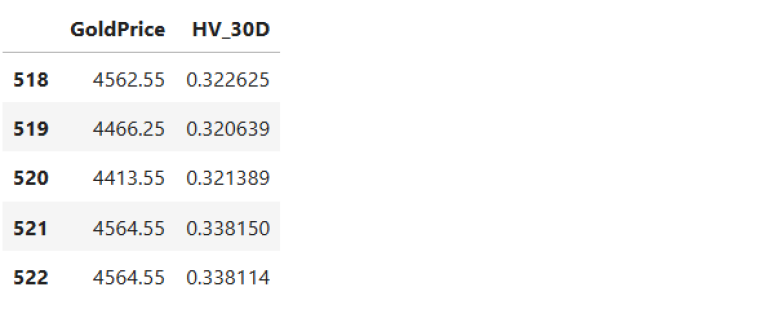
Step 2) Calculate Historical Volatility
- We compute daily returns → how much gold moves per day
- Then we calculate 30‑day rolling standard deviation → past variability
- Lastly, we multiply it by √252 → convert to annual volatility (There are usually about 252 trading days in a typical year)
# Step 2) Calculate Historical Volatility
# Extract price series
price = gold['Close Price'].astype(float)
# Daily percentage returns
returns = price.pct_change()
# 30‑day rolling historical volatility (annualized)
hist_vol_30d = returns.rolling(30).std() * (252 ** 0.5)
# Combine for inspection
vol_df = pd.concat([
price.rename('GoldPrice'),
hist_vol_30d.rename('HV_30D')
], axis=1)
display(vol_df.tail())
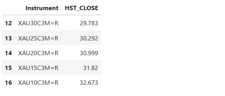
Step 3) Snapshot Implied Volatility (Using HST_CLOSE)
This gives us a point-in-time volatility smile — a powerful view into trader sentiment.
For LSEG-calculated instruments (RICs ending in =R), we're going to pick HST_CLOSE field as a snapshot IV field as this is the implied volatility “close” for that specific delta/tenor.
We load the full volatility smile:
# Step 3) Snapshot Implied Volatility (Using HST_CLOSE)
vol_rics = [
'XAU10P3M=R','XAU15P3M=R','XAU20P3M=R','XAU25P3M=R',
'XAU30P3M=R','XAU35P3M=R','XAU40P3M=R','XAU45P3M=R',
'XAU3MO=R',
'XAU45C3M=R','XAU40C3M=R','XAU35C3M=R','XAU30C3M=R',
'XAU25C3M=R','XAU20C3M=R','XAU15C3M=R','XAU10C3M=R'
]
iv_data = {}
iv = ld.get_data(
universe=vol_rics,
fields=['HST_CLOSE']
)
display(iv.tail())
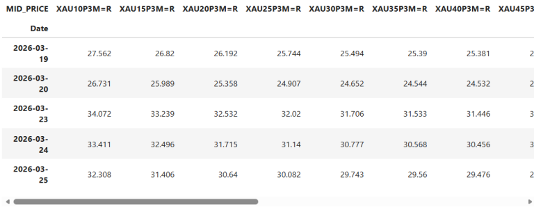
Step 4) Historical Implied Volatility (IV) Using MID_PRICE
The get_history() function of these RICs does not return HST_CLOSE field, so we use MID_PRICE (Midpoint between BID/ASK implied vol) for historical IV here as We want to compare how implied volatility evolves over time, so we need the historical series -- not just the snapshot.
# Step 4) Historical Implied Volatility (IV) Using MID_PRICE
iv_all = ld.get_history(
universe=vol_rics,
fields=['MID_PRICE'], # use MID_PRICE for IV history
interval='1D',
start=start,
end=end
)
display(iv_all.tail())
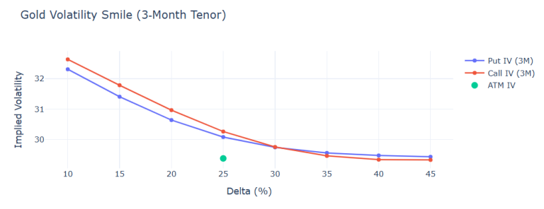
Step 5) Plot the Volatility Smile (Snapshot)
This shows how volatility varies across deltas.
You will now have a professional volatility smile that tells you the below
- High IV at low deltas = pricing of extreme moves
- Call IV slightly above put IV = safe-haven upside demand
- ATM vol = anchor of the curve
# Step 5) Plot the Volatility Smile (Snapshot)
latest = iv_all.dropna().iloc[-1]
deltas = [10,15,20,25,30,35,40,45]
put_vols = [latest[f"XAU{d}P3M=R"] for d in deltas]
call_vols = [latest[f"XAU{d}C3M=R"] for d in deltas[::-1]]
atm_vol = latest["XAU3MO=R"]
fig = go.Figure()
fig.add_trace(go.Scatter(
x=deltas, y=put_vols,
mode="lines+markers",
name="Put IV (3M)"
))
fig.add_trace(go.Scatter(
x=deltas, y=call_vols[::-1],
mode="lines+markers",
name="Call IV (3M)"
))
fig.add_trace(go.Scatter(
x=[25], y=[atm_vol],
mode="markers",
marker=dict(size=10),
name="ATM IV"
))
fig.update_layout(
title="Gold Volatility Smile (3‑Month Tenor)",
xaxis_title="Delta (%)",
yaxis_title="Implied Volatility",
template="plotly_white"
)
fig.show()
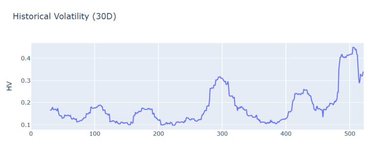
Step 6) Plot Historical Volatility (HV Only)
This chart acts like a “market turbulence monitor", which tells
- HV spikes around major events
- HV shows realized stress
- HV can be higher/lower than IV depending on market behavior
# Step 6) Plot Historical Volatility (HV Only)
fig = go.Figure()
fig.add_trace(go.Scatter(x=hist_vol_30d.index, y=hist_vol_30d))
fig.update_layout(title="Historical Volatility (30D)", yaxis_title="HV")
fig.show()
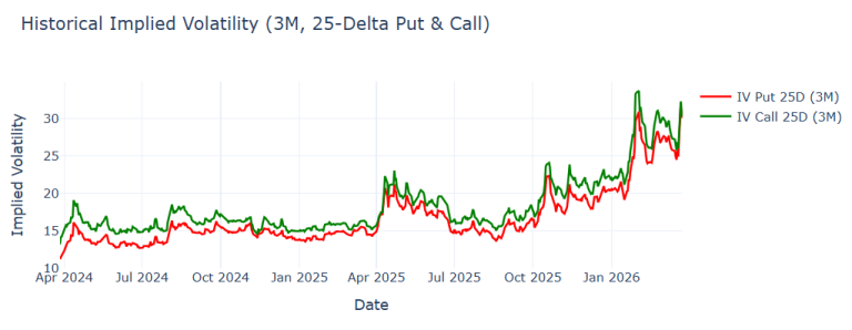
Step 7) Plot Historical Implied Vol (IV Only)
This time-series chart shows how expectations changed over the past 2 years.
- Put IV rises when traders fear downside
- Call IV rises when traders expect upside spikes
- Both rise when uncertainty grows
- Smooth seasonal patterns appear
Note: we plot this separately with HV Because HV ≈ 0.1–0.4 while IV ≈ 15–35, so this way is more clear and readable to visualize this data as they could not share a single y-axis scale.
# Step 7) Plot Historical Implied Vol (IV Only)
iv_put_25d = iv_all["XAU25P3M=R"].dropna()
iv_call_25d = iv_all["XAU25C3M=R"].dropna()
fig = go.Figure()
fig.add_trace(go.Scatter(
x=iv_put_25d.index,
y=iv_put_25d,
mode="lines",
name="IV Put 25D (3M)",
line=dict(color="red", width=2)
))
fig.add_trace(go.Scatter(
x=iv_call_25d.index,
y=iv_call_25d,
mode="lines",
name="IV Call 25D (3M)",
line=dict(color="green", width=2)
))
fig.update_layout(
title="Historical Implied Volatility (3M, 25-Delta Put & Call)",
xaxis_title="Date",
yaxis_title="Implied Volatility",
template="plotly_white"
)
fig.show()
Then, as a best practice, we close session that is being connected to the data platform.
ld.close_session()
Conclusion
Measuring gold volatility becomes much easier once you understand the different pieces that drive it. By combining historical volatility from gold fixing prices with the forward‑looking signals embedded in implied volatility, you gain a clearer picture of both what has happened in the market and what traders expect to happen next.
Historical volatility tells us how turbulent recent price movements have been, while implied volatility reflects the market’s anticipation of future uncertainty. Looking at implied volatility across put and call deltas reveals the volatility smile, which helps explain whether investors are more concerned about downside risks or upside spikes.
Separating historical volatility and implied volatility into different charts allows each to be seen clearly on its own scale, and makes it easier to spot patterns, shifts in sentiment, and moments where realized movements diverge from expectations. Together, these perspectives form a more complete understanding of gold’s behavior—something that is essential for anyone analyzing markets, managing risk, or working with derivatives.
Using the LSEG Data Library, we can retrieve, calculate, and visualize all of this data with just a few lines of code. This approach gives analysts and developers a powerful, flexible way to build dashboards, explore market dynamics, and better understand gold’s role as both an investment and a signal of global uncertainty.
If you continue exploring, you can expand this analysis into volatility skew, term structure, event‑driven volatility changes, or even automated monitoring dashboards. But even at this stage, you now have a strong foundation for understanding gold volatility—and the tools to track it confidently.
- Register or Log in to applaud this article
- Let the author know how much this article helped you
If you require assistance, please
contact us here
Get In Touch
Source Code
Related APIs
Related Articles
-
Gold Prices Are Surging - Here's How to Analyze Gold Miners with the LSEG Data Library
-
Check LSEG Data Library for Python Usage Limits Remaining
-
The Data Library for Python - Quick Reference Guide (Access layer)
-
Step-By-Step Guide to install Data Library for Python using Virtual Environment
-
LSEG Data Library for Python: News Pagination
-
LSEG’s Refinitiv Data Library for Python and its Configuration Process
Request Free Trial
Call your local sales team
Americas
All countries (toll free): +1 800 427 7570
Brazil: +55 11 47009629
Argentina: +54 11 53546700
Chile: +56 2 24838932
Mexico: +52 55 80005740
Colombia: +57 1 4419404
Europe, Middle East, Africa
Europe: +442045302020
Africa: +27 11 775 3188
Middle East & North Africa: 800035704182
Asia Pacific (Sub-Regional)
Australia & Pacific Islands: +612 8066 2494
China mainland: +86 10 6627 1095
Hong Kong & Macau: +852 3077 5499
India, Bangladesh, Nepal, Maldives & Sri Lanka:
+91 22 6180 7525
Indonesia: +622150960350
Japan: +813 6743 6515
Korea: +822 3478 4303
Malaysia & Brunei: +603 7 724 0502
New Zealand: +64 9913 6203
Philippines: 180 089 094 050 (Globe) or
180 014 410 639 (PLDT)
Singapore and all non-listed ASEAN Countries:
+65 6415 5484
Taiwan: +886 2 7734 4677
Thailand & Laos: +662 844 9576