
Updated: 28 Feb 2025
Overview
Technical Analysis for intraday trading is one of the basic approaches to help you choose the planning of ventures. Basically, users can use the intraday or end-of-day pricing data to generate charts such as the CandleStick. And then, they can review the stock price' trend and make decisions using their own mehtod or algorithm. Typically, LSEG Workspace and Eikon Desktop users also provide access to this information, and it also provides a user interface to display multiple types of Charts.
However, there is a specific requirement from a customer who did not use Eikon or LSEG Workspace. They need to build their own stand-alone application or generate the charts on their application using data from LSEG. The user is looking for the source of data or service to provide the intraday data for them in the REST API format. So they can integrate the service with their app.
To support the requirement client can use REST API provided by Data Platform that basically provides simple web-based API access to a broad range of content provided by LSEG. It can retrieve data such as News, ESG, Symbology, Streaming Price, and Historical Pricing. Users can get the intraday from the Historical Pricing service and then pass the data to any libraries that provided functionality to generate Charts. To help API users access content easier, LSEG also provides the LSEG Data Platform Libraries that provide a set of uniform interfaces providing the developer access to the Data Platform. We are currently providing an LSEG Data Platform Libraries for Python, TypeScript and .NET users. A general user and data scientists can leverage the library's functionality to retrieve data from the service, which basically provides the original response message from the service in JSON tabular format. The LSEG Data Library for Python will then convert the JSON tabular format to the pandas dataframe so that the user does not need to handle a JSON message and convert it manually. The user can use the dataframe with libraries such as mathplotlib and mplfinance to display the Charts.
In this example, I will show you how to use the LSEG Data Library for Python, request the intraday data from the Historical Pricing service, and then generate basic charts such as the Candle Stick charts. Basically, the Japanese candlestick chart commonly used to illustrate movements in the price of a financial instrument over time. It's popular in finance, and some technical analysis strategies use them to make trading decisions, depending on the candles' shape, color, and position.
Prerequisites
Follow instructions from Quick Start Guide to install LSEG Data Library for python.
pip install lseg-data
You must have an RDP Account or LSEG Workspace desktop application with permission to request data using Historical Pricing API.
Ensure that you have the following additional python libraries.
matplotlib, mplfinance, seaborn, ipympl
Getting Started using LSEG Data Library for python
The library supports the configuration file (lseg-data.config.json). The configuaration file can be modified to connect to the desktop session or data platform session.
Set the "app-key" property and set the default session to "desktop.workspace" to connect to the desktop session.
"sessions": {
"default": "desktop.workspace",
...
"desktop": {
"workspace": {
"app-key": "<APP KEY>"
}
}
}
Set the "app-key", "username", and "password" properties and set the default session to "platform.ldp" to connect to the data platform session.
"sessions": {
"default": "platform.ldp",
"platform": {
"ldp": {
"app-key": "YOUR APP KEY GOES HERE!",
"username": "YOUR LDP LOGIN OR MACHINE GOES HERE!",
"password": "YOUR LDP PASSWORD GOES HERE!"
},
...
}
Open the Session
Next step, we will import lseg.data libraries, set the configuration's location, and open the default session.
import os
os.environ["LD_LIB_CONFIG_PATH"] = "./"
import lseg.data as ld
from lseg.data.content import historical_pricing
from lseg.data.content.historical_pricing import Intervals
from lseg.data.content.historical_pricing import Adjustments
from lseg.data.content.historical_pricing import MarketSession
global ricName
ld.open_session()
<lseg.data.session.Definition object at 0x1a6cc2b0350 {name='workspace'}>
Retrieve Time Series data
After the session state is Open, we will use the historical_pricing.summaries.Definition interface to retrieve time series pricing Interday summaries data(i.e., bar data).
Definition(universe: 'StrStrings', interval: Union[str, lseg.data.content._intervals.Intervals] = None, start: 'OptDateTime' = None, end: 'OptDateTime' = None, adjustments: 'OptAdjustments' = None, sessions: 'OptMarketSession' = None, count: 'OptInt' = None, fields: 'StrStrings' = None, extended_params: 'ExtendedParams' = None) -> None
Actually, the implementation of this function will send HTTP GET requests to the historical pricing endpoints.
And the following details are possible values for interval and adjustment arguments.
Supported intervals:
- Interday intervals: Intervals.DAILY, Intervals.ONE_DAY, Intervals.WEEKLY, Intervals.MONTHLY, Intervals.THREE_MONTHS, Intervals.TWELVE_MONTHS, Intervals.YEARLY.
- Intraday intervals: Intervals.FIVE_MINUTES, Intervals.HOURLY, Intervals.MINUTE, Intervals.SIXTY_MINUTES, Intervals.TEN_MINUTES, Intervals.THIRTY_MINUTES
Supported value for adjustments:
- Adjustments.UNADJUSTED - Not apply both exchange/manual corrections and CORAX
- Adjustments.EXCHANGE_CORRECTION - Apply exchange correction adjustment to historical pricing
- Adjustments.MANUAL_CORRECTION - Apply manual correction adjustment to historical pricing, i.e. annotations made by content analysts
- Adjustments.CCH - Apply Capital Change adjustment to historical Pricing due to Corporate Actions e.g. stock split
- Adjustments.CRE - Apply Currency Redenomination adjustment when there is redenomination of currency
- Adjustments.RPO - Apply Reuters Price Only adjustment to adjust historical price only not volume
- Adjustments.RTS - Apply Reuters TimeSeries adjustment to adjust both historical price and volume
- Adjustments.QUALIFIERS - Apply price or volume adjustment to historical pricing according to trade/quote qualifier summarization actions
You can pass an array of these values to the function like the below sample codes.
adjustments = [
Adjustments.EXCHANGE_CORRECTION,
Adjustments.MANUAL_CORRECTION
]
The adjustments are a query parameter that tells the system whether to apply or not apply CORAX (Corporate Actions) events or exchange/manual corrections or price and volume adjustment according to trade/quote qualifier summarization actions to historical time series data.
Normally, the back-end should strictly serve what clients need. However, if the back-end cannot support them, the back-end can still return the form that the back-end supports with the proper adjustments in the response and status block (if applicable) instead of an error message.
Limitations: Adjustment behaviors listed in the limitation section may be changed or improved in the future.
If any combination of correction types is specified (i.e., exchangeCorrection or manualCorrection), all correction types will be applied to data in applicable event types.
If any combination of CORAX is specified (i.e., CCH, CRE, RPO, and RTS), all CORAX will be applied to data in applicable event types.
Adjustments values for Interday-summaries and Intraday-summaries API
If unspecified, each back-end service will be controlled with the proper adjustments in the response so that the clients know which adjustment types are applied by default. In this case, the returned data will be applied with exchange and manual corrections and applied with CORAX adjustments.
If specified, the clients want to get some specific adjustment types applied or even unadjusted.
Notes:
Summaries data will always have exchangeCorrection and manualCorrection applied. If the request is explicitly asked for uncorrected data, a status block will be returned along with the corrected data saying, "Uncorrected summaries are currently not supported".
The unadjusted will be ignored when other values are specified.
Below is a sample code to retrieve Daily historical pricing for the RIC defined in ricName variable, and I will set the start date from 2020 to nowaday. You need to set the interval to rdp.Intervals.DAILY to get intraday data. We will display the columns name with the heads and tails of the dataframe to review the data.
import pandas as pd
import datetime
from IPython.display import clear_output
pd.set_option('future.no_silent_downcasting', True)
ricName='MSFT.O'
StartDate = '2020.01.01'
EndDate = str(datetime.date.today())
response = historical_pricing.summaries.Definition(
universe = ricName,
interval = Intervals.DAILY, # Supported intervals: DAILY, WEEKLY, MONTHLY, QUARTERLY, YEARLY.
start = StartDate,
end = EndDate).get_data()
if response is not None:
#Show information of the dataframe to see column name , null and null-null field and the data type of the column
response.data.df.info()
display(response.data.df.head)
display(response.data.df.tail)
else:
print("Error while process the data")
Sample Output
<class 'pandas.core.frame.DataFrame'>
DatetimeIndex: 1296 entries, 2020-01-02 to 2025-02-27
Data columns (total 16 columns):
# Column Non-Null Count Dtype
--- ------ -------------- -----
0 TRDPRC_1 1296 non-null Float64
1 HIGH_1 1296 non-null Float64
2 LOW_1 1296 non-null Float64
3 ACVOL_UNS 1296 non-null Int64
4 OPEN_PRC 1296 non-null Float64
5 BID 1296 non-null Float64
6 ASK 1296 non-null Float64
7 TRNOVR_UNS 1296 non-null Float64
8 VWAP 1296 non-null Float64
9 BLKCOUNT 1296 non-null Int64
10 BLKVOLUM 1296 non-null Int64
11 NUM_MOVES 1296 non-null Int64
12 TRD_STATUS 1296 non-null Int64
13 SALTIM 1296 non-null Int64
14 NAVALUE 0 non-null Int64
15 VWAP_VOL 132 non-null Int64
dtypes: Float64(8), Int64(8)
memory usage: 192.4 KB
C:\Python311\Lib\site-packages\pandas\core\dtypes\cast.py:1057:RuntimeWarning: invalid value encountered in cast
C:\Python311\Lib\site-packages\pandas\core\dtypes\cast.py:1081:RuntimeWarning: invalid value encountered in cast
<bound method NDFrame.head of MSFT.O TRDPRC_1 HIGH_1 LOW_1 ACVOL_UNS OPEN_PRC BID ASK \
Date
2020-01-02 160.62 160.73 158.33 22634546 158.78 160.7 160.73
2020-01-03 158.62 159.945 158.06 21121681 158.32 158.59 158.6
2020-01-06 159.03 159.1 156.51 20826702 157.08 159.02 159.03
2020-01-07 157.58 159.67 157.32 21881740 159.32 157.57 157.59
2020-01-08 160.09 160.8 157.9491 27762026 158.93 160.13 160.14
... ... ... ... ... ... ... ...
2025-02-21 408.21 418.048 407.89 27524799 417.335 408.13 408.21
2025-02-24 404.0 409.37 399.32 26443656 408.51 404.01 404.09
2025-02-25 397.9 401.915 396.7 29387402 401.1 397.89 398.0
2025-02-26 399.73 403.6 394.245 19618954 398.01 399.64 399.73
2025-02-27 392.53 405.74 392.17 21127406 401.265 392.57 392.62
MSFT.O TRNOVR_UNS VWAP BLKCOUNT BLKVOLUM NUM_MOVES \
Date
2020-01-02 3616467558.697274 159.7217 48 5316243 175502
2020-01-03 3362128402.01136 159.2274 40 4912883 166450
2020-01-06 3300691292.711478 158.4213 39 6565484 148389
2020-01-07 3463850960.600081 158.343 39 5082001 167836
2020-01-08 4430819413.553828 159.6757 45 6642775 198630
... ... ... ... ... ...
2025-02-21 11326060877.0 411.5663 73 12664561 385141
2025-02-24 10668937055.0 403.1559 59 7604321 514485
2025-02-25 11722702308.0 398.8885 76 10602443 492990
2025-02-26 7840275351.0 400.0295 45 7471141 327110
2025-02-27 8370743495.0 396.3325 38 6753730 377155
MSFT.O TRD_STATUS SALTIM NAVALUE VWAP_VOL
Date
2020-01-02 1 75600 <NA> <NA>
2020-01-03 1 75600 <NA> <NA>
2020-01-06 1 76500 <NA> <NA>
2020-01-07 1 76500 <NA> <NA>
2020-01-08 1 75600 <NA> <NA>
... ... ... ... ...
2025-02-21 1 76500 <NA> 22708867
2025-02-24 1 75600 <NA> 22324366
2025-02-25 1 75600 <NA> 24785038
2025-02-26 1 75600 <NA> 13872096
2025-02-27 1 75600 <NA> 17193205
[1296 rows x 16 columns]>
<bound method NDFrame.tail of MSFT.O TRDPRC_1 HIGH_1 LOW_1 ACVOL_UNS OPEN_PRC BID ASK \
Date
2020-01-02 160.62 160.73 158.33 22634546 158.78 160.7 160.73
2020-01-03 158.62 159.945 158.06 21121681 158.32 158.59 158.6
2020-01-06 159.03 159.1 156.51 20826702 157.08 159.02 159.03
2020-01-07 157.58 159.67 157.32 21881740 159.32 157.57 157.59
2020-01-08 160.09 160.8 157.9491 27762026 158.93 160.13 160.14
... ... ... ... ... ... ... ...
2025-02-21 408.21 418.048 407.89 27524799 417.335 408.13 408.21
2025-02-24 404.0 409.37 399.32 26443656 408.51 404.01 404.09
2025-02-25 397.9 401.915 396.7 29387402 401.1 397.89 398.0
2025-02-26 399.73 403.6 394.245 19618954 398.01 399.64 399.73
2025-02-27 392.53 405.74 392.17 21127406 401.265 392.57 392.62
MSFT.O TRNOVR_UNS VWAP BLKCOUNT BLKVOLUM NUM_MOVES \
Date
2020-01-02 3616467558.697274 159.7217 48 5316243 175502
2020-01-03 3362128402.01136 159.2274 40 4912883 166450
2020-01-06 3300691292.711478 158.4213 39 6565484 148389
2020-01-07 3463850960.600081 158.343 39 5082001 167836
2020-01-08 4430819413.553828 159.6757 45 6642775 198630
... ... ... ... ... ...
2025-02-21 11326060877.0 411.5663 73 12664561 385141
2025-02-24 10668937055.0 403.1559 59 7604321 514485
2025-02-25 11722702308.0 398.8885 76 10602443 492990
2025-02-26 7840275351.0 400.0295 45 7471141 327110
2025-02-27 8370743495.0 396.3325 38 6753730 377155
MSFT.O TRD_STATUS SALTIM NAVALUE VWAP_VOL
Date
2020-01-02 1 75600 <NA> <NA>
2020-01-03 1 75600 <NA> <NA>
2020-01-06 1 76500 <NA> <NA>
2020-01-07 1 76500 <NA> <NA>
2020-01-08 1 75600 <NA> <NA>
... ... ... ... ...
2025-02-21 1 76500 <NA> 22708867
2025-02-24 1 75600 <NA> 22324366
2025-02-25 1 75600 <NA> 24785038
2025-02-26 1 75600 <NA> 13872096
2025-02-27 1 75600 <NA> 17193205
[1296 rows x 16 columns]>
Preparing data for plotting chart
Next steps, we will create a new dataframe object from the data returned by the interday-summaries endpoint. We need to map the columns from the original dataframe to Open, High, Low, Close(OHLC) data. So we will define column names to map the OHLC data from the following variables.
openColumns =>Open
highColumns => High
lowColumns => Low
closeColumns => Close
volumeColums => Volume
openColumns="OPEN_PRC"
highColumns="HIGH_1"
lowColumns="LOW_1"
closeColumns="TRDPRC_1"
volumeColumns="ACVOL_UNS"
ohlc_dataframe= data[[openColumns,highColumns,lowColumns,closeColumns,volumeColumns]]
ohlc_dataframe.index.name = 'Date'
display(ohlc_dataframe)
#rename the column name
ohlc_dataframe.info()
ohlc_dataframe=ohlc_dataframe.rename(columns={openColumns:"Open",highColumns:"High",lowColumns:"Low",closeColumns:"Close",volumeColumns:"Volume"})
print(ohlc_dataframe.columns)
display(ohlc_dataframe)
Sample Output
MSFT.O OPEN_PRC HIGH_1 LOW_1 TRDPRC_1 ACVOL_UNS
Date
2020-01-02 158.78 160.73 158.33 160.62 22634546
2020-01-03 158.32 159.945 158.06 158.62 21121681
2020-01-06 157.08 159.1 156.51 159.03 20826702
2020-01-07 159.32 159.67 157.32 157.58 21881740
2020-01-08 158.93 160.8 157.9491 160.09 27762026
... ... ... ... ... ...
2025-02-21 417.335 418.048 407.89 408.21 27524799
2025-02-24 408.51 409.37 399.32 404.0 26443656
2025-02-25 401.1 401.915 396.7 397.9 29387402
2025-02-26 398.01 403.6 394.245 399.73 19618954
2025-02-27 401.265 405.74 392.17 392.53 21127406
1296 rows × 5 columns
<class 'pandas.core.frame.DataFrame'>
DatetimeIndex: 1296 entries, 2020-01-02 to 2025-02-27
Data columns (total 5 columns):
# Column Non-Null Count Dtype
--- ------ -------------- -----
0 OPEN_PRC 1296 non-null Float64
1 HIGH_1 1296 non-null Float64
2 LOW_1 1296 non-null Float64
3 TRDPRC_1 1296 non-null Float64
4 ACVOL_UNS 1296 non-null Int64
dtypes: Float64(4), Int64(1)
memory usage: 67.1 KB
Index(['Open', 'High', 'Low', 'Close', 'Volume'], dtype='object', name='MSFT.O')
MSFT.O Open High Low Close Volume
Date
2020-01-02 158.78 160.73 158.33 160.62 22634546
2020-01-03 158.32 159.945 158.06 158.62 21121681
2020-01-06 157.08 159.1 156.51 159.03 20826702
2020-01-07 159.32 159.67 157.32 157.58 21881740
2020-01-08 158.93 160.8 157.9491 160.09 27762026
... ... ... ... ... ...
2025-02-21 417.335 418.048 407.89 408.21 27524799
2025-02-24 408.51 409.37 399.32 404.0 26443656
2025-02-25 401.1 401.915 396.7 397.9 29387402
2025-02-26 398.01 403.6 394.245 399.73 19618954
2025-02-27 401.265 405.74 392.17 392.53 21127406
1296 rows × 5 columns
Visualizing Stock Data
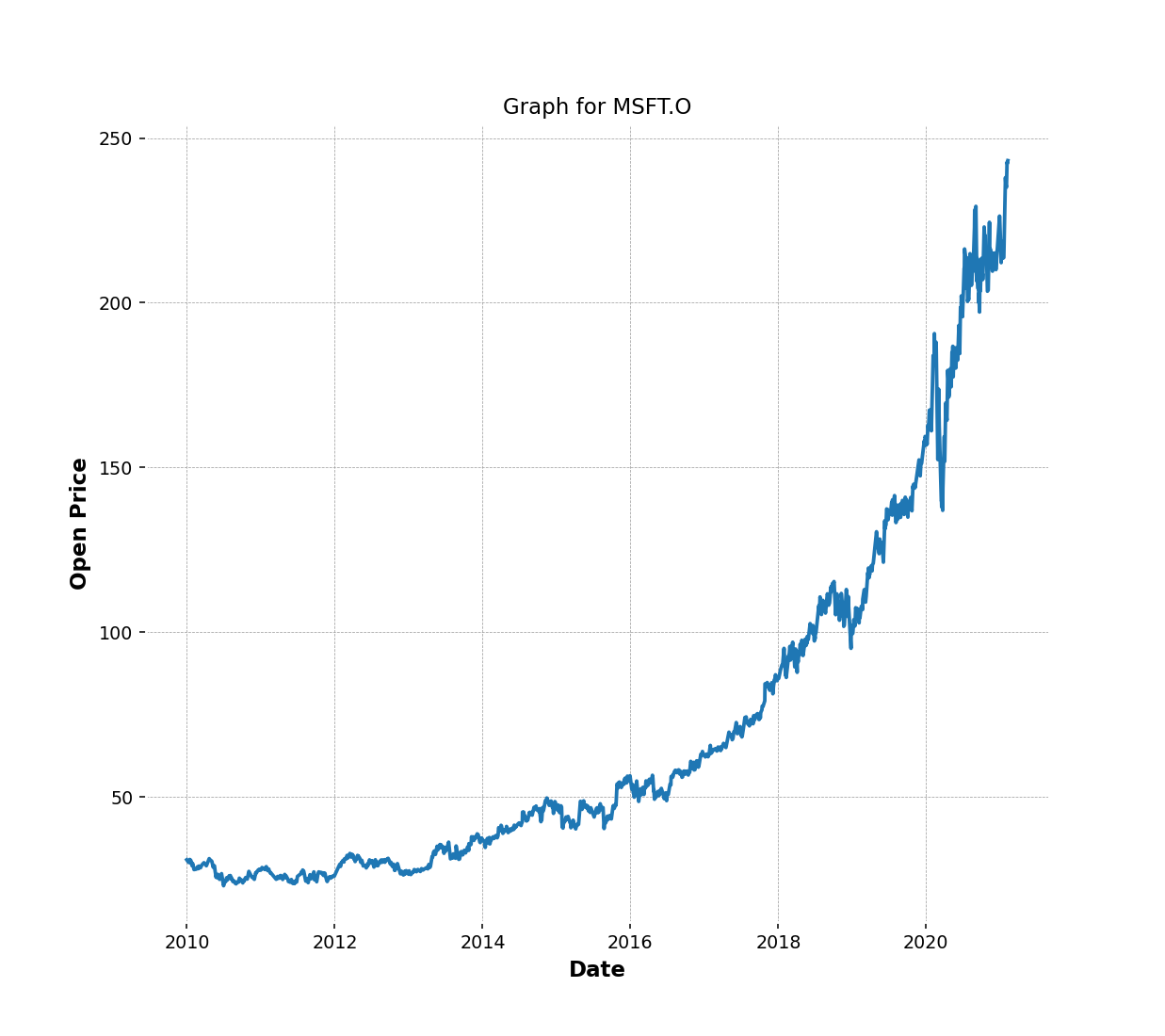
Plot a simple Daily Closing Price line graph
We can create a simple line graph to compare open and close price using the following codes. You can change the size of the figure.figsize to adjust chart size.
import matplotlib.pyplot as plt
%matplotlib ipympl
fig = plt.figure(figsize=(9,8),dpi=100)
ax = plt.subplot2grid((3,3), (0, 0), rowspan=3, colspan=3)
titlename='Graph for '+ricName
ax.set_title(titlename)
ax.set_xlabel('Date')
ax.set_ylabel('Open Price')
ax.grid(True)
ax.plot(ohlc_dataframe.index, ohlc_dataframe.Open)
plt.show()
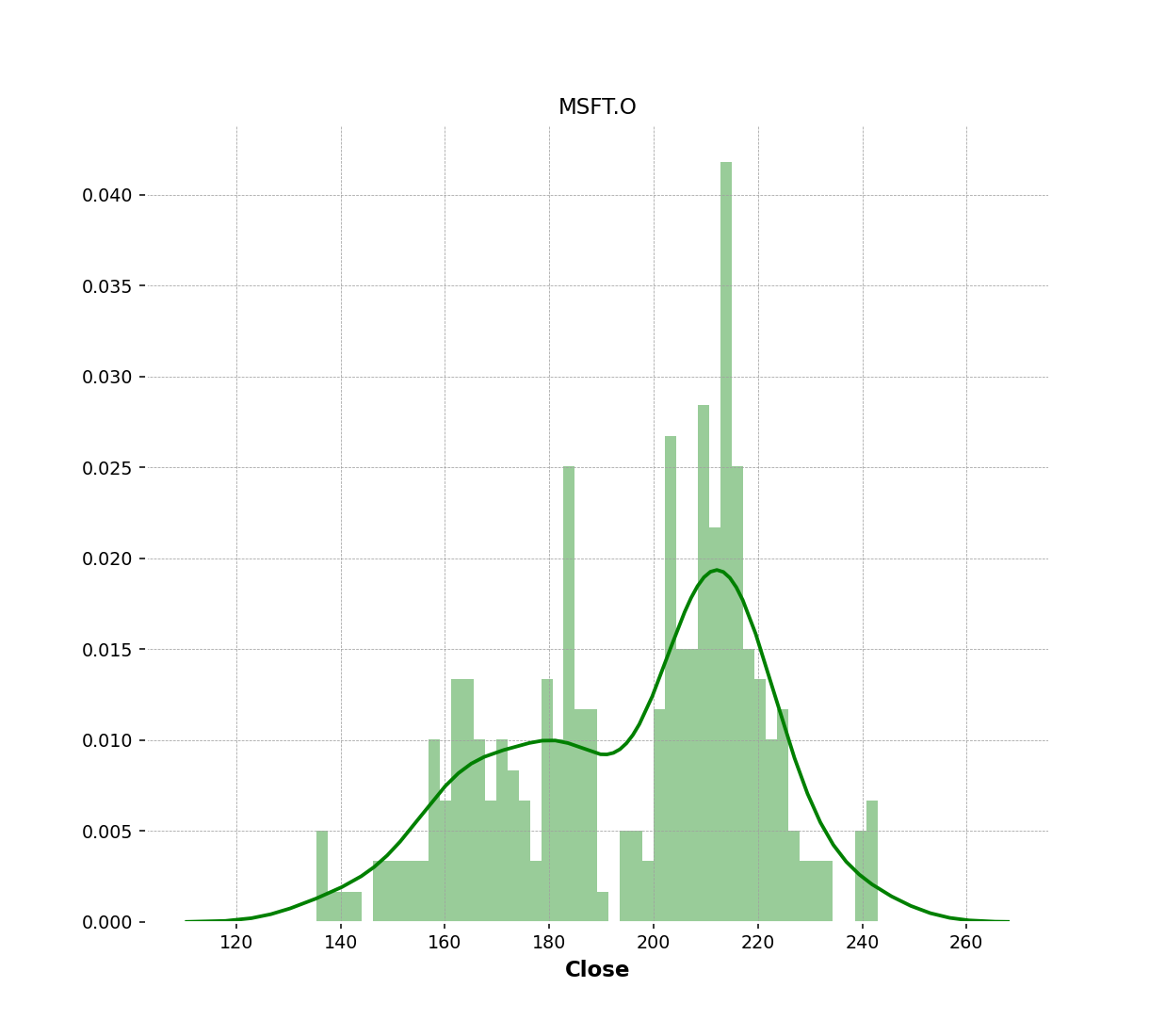
Generate a Histogram of the Daily Closing Price
We can review daily closing prices over time to see the spread or volatility and the type of distribution using the histogram. We can use the histplot method from the seaborn library to plot the graph.
import seaborn as sns
import matplotlib.pyplot as plt
plt.figure(figsize=(9,8),dpi=100)
dfPlot=ohlc_dataframe[['Close','Volume']].loc['2020-01-01':datetime.date.today(),:]
graph=sns.histplot(dfPlot.Close.dropna(),
bins=50,
color='green',
kde=True,
stat="density",
kde_kws=dict(cut=3))
graph.set(title=ricName)
plt.show()
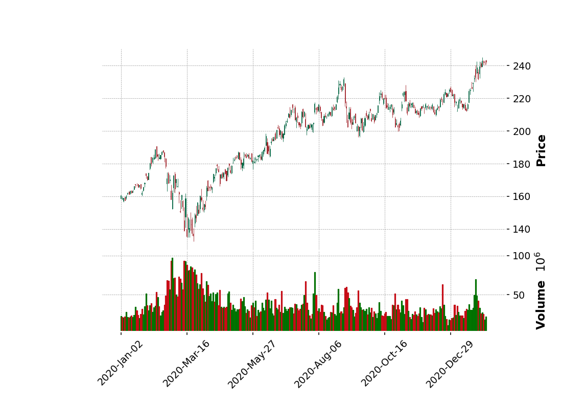
Using the mplfiance library to generate CandleStick and OHLC chart
Next step, we will generate a CandleStick and OHLC chart using the new version mplfinance library. We need to pass a dataframe that contains Open, High, Low, and Close data to the mplfinance.plot function and specify the name of the chart you want to plot.
import mplfinance as mpf
import datetime
%matplotlib ipympl
ohlc_dataframe.info()
#Volume use Int64 it will returns fails when mplfinance.plot check the support type of the data.So we need to convert it to Int64 and remove na from the data frame.
#If you don't care about Volume you can drop it from the dataframe.
dfPlot=ohlc_dataframe.dropna().astype({col: 'int64' for col in ohlc_dataframe.select_dtypes('Int64').columns}).loc['2024-01-01':str(datetime.date.today())]
display(dfPlot)
dfPlot.info()
mpf.plot(dfPlot.loc[:str(datetime.date.today()),:],type='candle',style='charle
Display shorter period.
tempPlot= ohlc_dataframe.dropna().astype({col: 'int64' for col in ohlc_dataframe.select_dtypes('Int64').columns}).loc['2025-01-01':str(datetime.date.today())]
mpf.plot(tempPlot,type='candle',style='charles',volume=True)
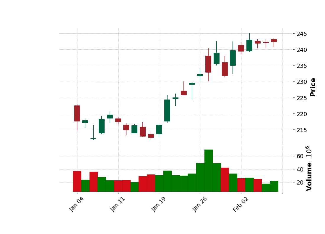
From a candlestick chart(zoom the graph), a green candlestick indicates a day where the closing price was higher than the open(Gain), while a red candlestick indicates a day where the open was higher than the close (Loss). The wicks indicate the high and the low, and the body the open and close (hue is used to determine which end of the body is open and which the close). You can follow the instruction from the following example to change the color. You need to pass your own style to the plot function. And as I said previously, a user can use Candlestick charts for technical analysis and use them to make trading decisions, depending on the candles' shape, color, and position. We will not cover a technical analysis in this example.
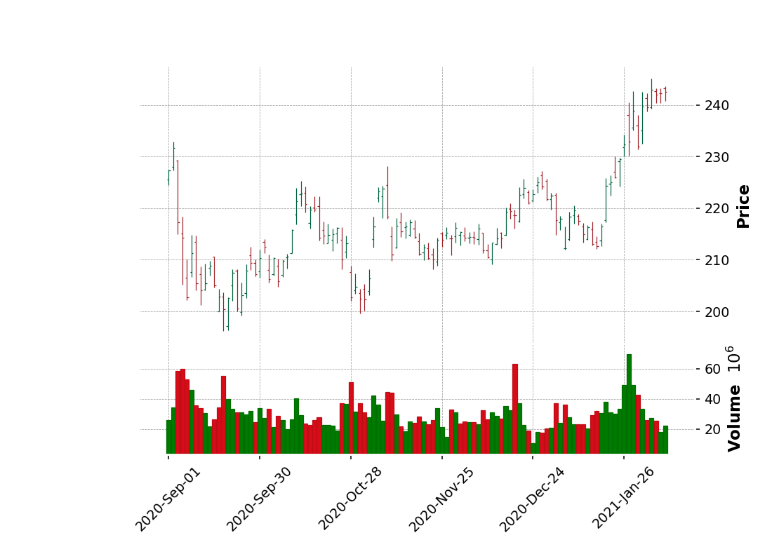
Plot OHLC chart
An OHLC chart is a type of bar chart that shows open, high, low, and closing prices for each period. OHLC charts are useful since they show the four major data points over a period, with the closing price being considered the most important by many traders. The chart type is useful because it can show increasing or decreasing momentum. When the open and close are far apart, it shows strong momentum, and when they open and close are close together, it shows indecision or weak momentum. The high and low show the full price range of the period, useful in assessing volatility. There several patterns traders watch for on OHLC charts [8].
To plot the OHLC chart, you can just change the type to 'ohlc'. It's quite easy when using mplfinance.
mpf.plot(dfPlot.loc['2024-09-01':str(datetime.date.today()),:],type='ohlc',style='charles',volume=True)
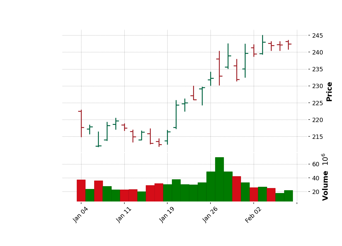
display(dfPlot)
mpf.plot(dfPlot.loc['2025-01-01':str(datetime.date.today()),:],type='ohlc',style='charles',volume=True)
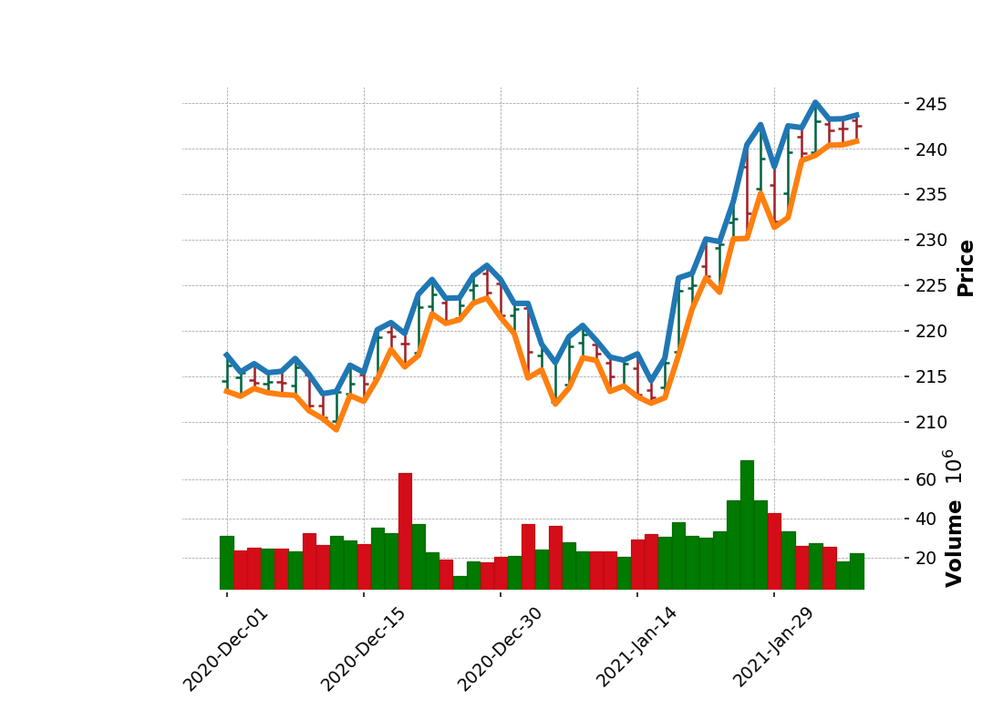
Adding plots to the basic mplfinance plot()
Sometimes you may want to plot additional data within the same figure as the basic OHLC or Candlestick plot. For example, you may want to add the results of a technical study or some additional market data.
This is done by passing information into the call to mplfinance.plot() using the addplot ("additional plot") keyword. I will show you a sample of the additional plots by adding a line plot for the data from columns High and Low to the original OHLC chart.
dfSubPlot = dfPlot.loc['2024-12-01':str(datetime.date.today()),:]
apdict = mpf.make_addplot(dfSubPlot[['High','Low']])
mpf.plot(dfSubPlot,type='ohlc',style='charles',volume=True,addplot=apdict)
Add Simple Moving Average to the Chart
Next steps, we will add a moving average (MA) to the CandleStick chart. MA is widely used as the technical analysis indicator that helps smooth out price action by filtering out the “noise” from random short-term price fluctuations. It is a trend-following or lagging indicator because it is based on past prices. The two basic and commonly used moving averages are the simple moving average (SMA), the simple average of a security over a defined number of time periods, and the exponential moving average (EMA), giving greater weight to more recent prices. Note that this example will use only built-in MA provided by the mplfinance. The most common moving averages are to identify the trend direction and determine support and resistance levels.
Basically, mplfinance provides functionality for easily computing a moving average. The following codes creating a 20-day moving average from the price provided in the dataframe, and plotting it alongside the stock. Moving averages lag behind current price action because they are based on past prices; the longer the time period for the moving average, the greater the lag. Thus, a 200-day MA will have a much greater degree of lag than a 20-day MA because it contains prices for the past 200 days.
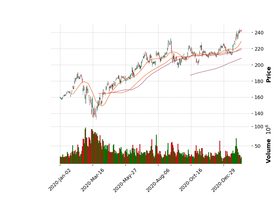
mpf.plot(dfPlot.loc[:str(datetime.date.today()),:],type='candle',style='charles',mav=(20),volume=True)
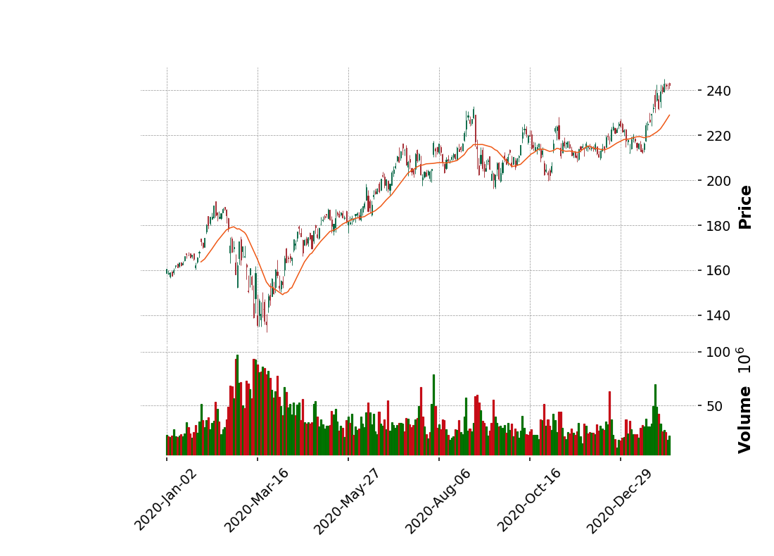
The length of the moving average to use depends on the trading objectives, with shorter moving averages used for short-term trading and longer-term moving averages more suited for long-term investors. The 50-day and 200-day MAs are widely followed by investors and traders, with breaks above and below this moving average considered important trading signals.
The following codes use to generated CandleStick charts with multiple periods of times for SMA (20-day,50-day,75-day, and 200-day).
mpf.plot(dfPlot.loc[:str(datetime.date.today()),:],type='candle',style='charles',mav=(20,60,75,200),volume=True)
Zoom the chart to display shorter period.
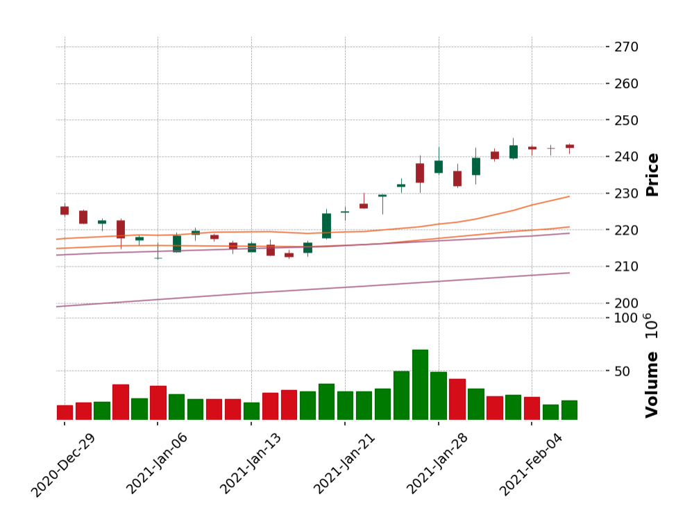
You can also calculate the moving average from your own method or algorithm using the original data from the dataframe and then add a subplot to the CandleStick charts using add plot like the previous sample of OHLC charts.
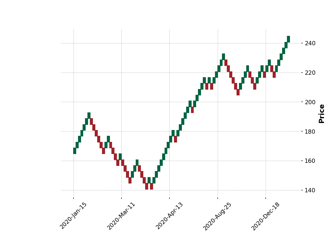
Generate Renko Chart
Based on the investopedia page, a Renko chart is a type of chart developed by the Japanese that is built using price movement rather than both price and standardized time intervals like most charts are. It is thought to be named after the Japanese word for bricks, "renga," since the chart looks like a bricks series. A new brick is created when the price moves a specified price amount, and each block is positioned at a 45-degree angle (up or down) to the prior brick. An up brick is typically colored white or green, while a down brick is typically colored black or red[7].
Renko charts filter out the noise and help traders more clearly see the trend since all smaller movements than the box size are filtered out.Renko charts typically only use closing prices based on the chart time frame chosen. For example, if using a weekly time frame, weekly closing prices will be used to construct the bricks[7].
mpf.plot(dfPlot,type='renko',style='charles',renko_params=dict(brick_size=4))
Summary
This article explains users' alternate choices to retrieve such kind of the End of Day price or intraday datatime series data from the LSEG Data Libaray for Python. This article provides a sample code to use the LSEG Data Library for python to retrieve the Historical Pricing service, and then shows how to utilize the data with the 3rd party library such as the mplfinance to plot charts like the CandleStick, OHLC, and Renko chart for stock price technical analysis. With the library, users can specify a different kind of interval and adjustment behavior to retrieve more specific data and visualize the data on various charts. They can then use the charts to identify trading opportunities in price trends and patterns seen on charts.