Author:

Accessing LinkUp in Refinitiv Quantitative Analytics
Refinitiv's Refinitiv Quantitative Analytics recently released an exciting new alternative data set, LinkUp. LinkUp keeps track of jobs posted and removed by the hiring company in the form of a daily time series. These companies are mapped to Refinitiv's PermID for easy inoperability between content sets. This article will begin by showing you how to access Refinitiv Quantitative Analytics with Python code, query the LinkUp Active Jobs and load it into a pandas dataframe.
StarMine Observations of LinkUp Active Job Postings Changes and Analyst Revisions
Before LinkUp alternative data was released to our customers, the StarMine Research team had the opportunity to explore the data. An interesting phenomenon we observed was that around the time the company experienced a significant change in jobs (i.e. many added or many removed), the analysts would revise their estimates accordingly in the same direction. The most promising case would obviously be when analyst revisions follow a significant active job postings change a few days or weeks later. However, though there were a lot of cases like that, it was not always so. Sometimes the analyst revisions preceded the active job postings change and sometimes they both changed in tandem.
Hence, we didn't presume that sell-side analysts were watching job postings activity and revising accordingly. Instead our intuition was that the job postings change was a manifestation of the company's view on its future prospects. Perhaps a reaction to a recent event or anticipation of an upcoming event. Either way, we suspect that the analyst revisions occur when analysts finally learn what the company already knows. So when one observes a significant change in active job postings, it's important to check whether analysts have already revised in the same direction. If not, they may very well soon!
Combining LinkUp with I/B/E/S Consensus Estimates and StarMine SmartEstimates
Following the code to pull LinkUp data from Refinitiv Quantitative Analytics, there will be similar code demonstrating how to do the same for Institutional Brokers Estimate System (I/B/E/S) Consensus Estimates and StarMine SmartEstimates. Then some code to analyze those three content sets together to demonstrate the relationship between a company changing the number of active job postings and analysts revising their estimates.
Contents
- Install and Import Libraries
- Connect to Refinitiv Quantitative Analytics
- Pick a Company / Measure / Period to focus on
- Translate company's PermID to LinkUp CompanyID
- Pull daily jobs time series
- Using the Company's PermID to lookup Estimate PermIDs
- Use Estimate PermID to pull I/B/E/S Consensus Estimates
- Pull the StarMine SmartEstimates
- Plot the LinkUp Active Job Postings against the I/B/E/S Consensus Estimates and the StarMine SmartEstimates
- Analyst Awareness
- Generalisation
- EPS estimates
- Look at Revenue estimates
- Conclusion
- References
Install and Import Libraries
I'm a big fan of using sqlalchemy for all flavors of database connections. Easy to use and works nicely with pandas. Note that - in Jupyter Notebook - you can execute Terminal commands in the notebook cells by prepending an exclamation point/bang( ! ) to the beginning of the command. This can be useful for many things such as getting information without having to open a Terminal/Command Prompt, or installing a conda package you are trying to use.
!pip install matplotlib pyodbc sqlalchemy
import datetime
import matplotlib
import matplotlib.dates as mdates
import matplotlib.pyplot as plt
import pandas as pd
import pyodbc
import sqlalchemy
from sqlalchemy import create_engine # ' create_engine ' is a sub library that we can use to connect to our server.
for w,z in zip(["matplotlib", "pandas", "sqlalchemy"], [matplotlib, pd, sqlalchemy]): # ' datetime' and ' pyodbc ' do not have '.__version__'s
print("The Python library " + w + " used here is version " + z.__version__)
pd.options.display.max_columns = 0 # This line stops Pandas from truncating columns.
The Python library matplotlib used here is version 3.3.3
The Python library pandas used here is version 1.1.4
The Python library sqlalchemy used here is version 1.3.20
Connect to Refinitiv Quantitative Analytics
Note that you'll have to use your own username and password. You may request for product details to get such credentials here
The server listed below is a Refinitiv Quantitative Analytics trial server. It's possible you may be assigned a different server.
server = 'c5zjhr0qacpdeus2mi4a01.public.dabc3424290b.database.windows.net' # This is the Refinitiv Quantitative Analytics trial server. It's possible you may be assigned a different server.
port = '3342' # This is the port that was assigned to you, think of it as an extension to the server address provided.
database = 'qai' # Within the Refinitiv Quantitative Analytics database to which you have access, there are many databases - we are interested in the 'qai' one.
username = '1a.john.smith'
password = 'enterpassword'
# Refinitiv Quantitative Analytics requires an encrypted connection, so the "Encryption=Yes" part is very important
(connection_str) = ("mssql+pyodbc://" + username +
":" + password + "@" + server +
":" + port + "/" + database +
"?driver=sql server?Encryption=Yes")
connection_str
'mssql+pyodbc://1a.john.smith:enterpassword@c5zjhr0kufiwpos2mi4t01.public.daeb3426290b.database.windows.net:3342/qai?driver=sql server?Encryption=Yes'
mssql_eng = create_engine(connection_str)
mssql_eng.connect()
<sqlalchemy.engine.base.Connection at 0x1f00a38e908>
Pick a Company / Measure / Period to focus on
We're looking at BP, but feel free to change the PermID to another company if you want.
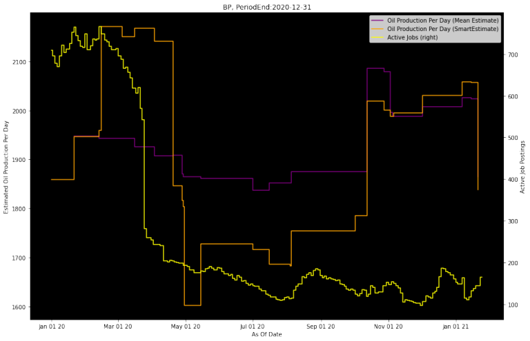
We're going to start by looking at an Industry Key Performance Indicators (KPIs), Oil Production Per Day, from I/B/E/S and StarMine SmartEstimates. Examples for Revenue and Earnings Per Share (EPS) are towards the end of this article.
orgpermid = 4295894740 # BP's Organization PermID
period_end = '2020-12-31'
period_type = 4 # Annual
measure = 164 # Measure code for Oil Production Per Day
measure_name = 'Oil Production Per Day' # For human-friendly chart labels
plot_date_start = '2020-01-01'
plot_date_end = '2021-01-26'
lookback_days = 30 # The change window for the Analyst Awareness metric
def lookup_companyid(orgpermid, plot_date_start):
# Let's setup our SQL query in the string ' companyid_sql ':
companyid_sql = f"""
SELECT CompanyID, CompanyName
FROM qai2.dbo.LinkUpCmpInfo
WHERE LUOrgPermID='{orgpermid}'
AND StartDate<='{plot_date_start}'
AND (EndDate>='{plot_date_start}' OR EndDate IS NULL)
"""
# Now let's collect our ' companyid_sql ' query with our authenticated connection ' mssql_eng ':
companyid_df = pd.read_sql(sql = companyid_sql,
con = mssql_eng)
# Now we can retrieve the information we are looking for from the reverted data:
companyid = companyid_df.iloc[0]['CompanyID']
company_name = companyid_df.iloc[0]['CompanyName']
return (companyid, company_name)
# Lookup LinkUp CompanyID for PermID
(companyid, company_name) = lookup_companyid(orgpermid, plot_date_start)
(companyid, company_name)
(3131, 'BP')
Pull daily jobs time series
Note that - in that function - we will need to strongly type our date. Strongly typed is a concept used to refer to a programming language that enforces strict restrictions on intermixing of values with differing data types. When such restrictions are violated and error (exception) occurs
def grab_linkup_data(companyid):
# Let's setup our SQL query in the string ' linkup_sql ':
linkup_sql = f"""
SELECT *
FROM qai2.dbo.LinkUpCmpAnalytics
WHERE CompanyID={companyid}
"""
# Now let's collect our ' linkup_sql ' query with our authenticated connection ' mssql_eng ':
linkup_df = pd.read_sql(linkup_sql, mssql_eng)
# Strongly type the date for charting in pandas later on
linkup_df['Date_'] = pd.to_datetime(linkup_df['Date_']).dt.date
return linkup_df
linkup_df = grab_linkup_data(companyid)
# We're going to focus on UniqueActiveJobCount in later code
linkup_df.tail()
| CompanyID | Date_ | CreatedJobCount | DeletedJobCount | UniqueActiveJobCount | ActiveDuration | |
| 4680 | 3131 | 27/08/2019 | 0 | 0 | 575 | 33.511299 |
| 4681 | 3131 | 28/08/2019 | 39 | 29 | 585 | 32.635899 |
| 4682 | 3131 | 29/08/2019 | 0 | 0 | 585 | 33.6171 |
| 4683 | 3131 | 30/08/2019 | 19 | 0 | 604 | 33.541401 |
| 4684 | 3131 | 31/08/2019 | 15 | 34 | 585 | 34.148701 |
def lookup_estimateid(orgpermid, plot_date_start):
# Let's setup our SQL query in the string ' perm_sql ':
perm_sql = f"""
SELECT EstPermID
FROM qai.dbo.TREInfo
WHERE OrgPermID={orgpermid}
AND EffectiveDate<='{plot_date_start}'
AND (ExpireDate>='{plot_date_start}' OR ExpireDate IS NULL)
"""
# Now let's collect our ' perm_sql ' query with our authenticated connection ' mssql_eng ':
perm_df = pd.read_sql(perm_sql, mssql_eng)
# Now we can retrieve the information we are looking for from the reverted data:
estimateid = perm_df.iloc[0]['EstPermID']
return estimateid
# Lookup EstimateID for LinkUp Stock_Ticker
estimateid = lookup_estimateid(orgpermid, plot_date_start)
estimateid
30064789400
Use Estimate PermID to pull I/B/E/S Consensus Estimates
Now that we have Estimate PermID, we can pull the I/B/E/S Consensus Estimates. We're only pulling data for one period, but there's tons more data in Refinitiv Quantitative Analytics.
Note that I'm "dumbing down" the time series to be daily. It's really intraday, since the consensus is updated as analysts update their individual estimates throughout the day. But the LinkUp Active Jobs Count is daily, so it's easier to plot a daily time series vs. a daily time series. Hence, I'm just going to take the last consensus estimate on a given day. But know that the full data is much more granular!
def grab_ibes_data(estimateid, measure, period_end, period_type):
# Let's setup our SQL query in the string ' ibes_sql ':
ibes_sql = f"""
WITH intraday
AS
(
-- Focus on one Security / Measure / PeriodEndDate / Periodicity
SELECT *
FROM qai.dbo.TRESumPer
WHERE EstPermID = {estimateid}
AND Measure = {measure}
AND PerEndDate = '{period_end}'
AND PerType = {period_type}
),
day_ends
AS
(
-- Dailyize the intraday time series by picking the last estimate of the day
SELECT CONVERT(DATE, EffectiveDate) AS AsOfDate, MAX(EffectiveDate) AS LastTime
FROM intraday
GROUP BY CONVERT(DATE, EffectiveDate)
)
SELECT d.AsOfDate, i.*
FROM intraday i
INNER JOIN day_ends d
ON i.EffectiveDate = d.LastTime
ORDER BY i.EffectiveDate
"""
# Now let's collect our ' ibes_sql ' query with our authenticated connection ' mssql_eng ':
ibes_df = pd.read_sql(ibes_sql, mssql_eng)
# Strongly type the date for charting in pandas later on
ibes_df['AsOfDate'] = pd.to_datetime(ibes_df['AsOfDate']).dt.date
return ibes_df
ibes_df = grab_ibes_data(estimateid, measure, period_end, period_type)
ibes_df.tail()
| AsOfDate | EstPermID | Measure | IsParent | PerType | PerEndDate | FYEMonth | EffectiveDate | EffectiveOffset | ExpireDate | ExpireOffset | ActivationDate | IsRealtime | DefStdDev | DefHighEst | DefLowEst | DefMeanEst | DefMedianEst | DefCurrPermID | DefScale | UnitType | NormStdDev | NormHighEst | NormLowEst | NormMeanEst | NormMedianEst | NormCurrPermID | NormScale | NormSplitFactor | NormCurrAdj | MarginPct | NumIncEsts | NumEsts | RegionPermID | |
| 62 | 05/11/2020 | 30064789400 | 164 | FALSE | 4 | 00:00.0 | 12 | 16:00.0 | 0 | 20:00.0 | 0 | 11:40.1 | TRUE | 28.64728 | 2027 | 1959 | 1988 | 1978 | 0 | 1000 | Barrels | 28.64728 | 2027 | 1959 | 1988 | 1978 | 0 | 1000 | 1 | 1 | None | 3 | 4 | 110172 |
| 63 | 02/12/2020 | 30064789400 | 164 | FALSE | 4 | 00:00.0 | 12 | 20:00.0 | 0 | 02:00.0 | 0 | 18:45.6 | TRUE | 55.93051 | 2086 | 1959 | 2007.66667 | 1978 | 0 | 1000 | Barrels | 55.93051 | 2086 | 1959 | 2007.66667 | 1978 | 0 | 1000 | 1 | 1 | None | 3 | 4 | 110172 |
| 64 | 07/01/2021 | 30064789400 | 164 | FALSE | 4 | 00:00.0 | 12 | 02:00.0 | 0 | 19:00.0 | 0 | 36:28.5 | TRUE | 58.39735 | 2086 | 1959 | 2026.5 | 2030.5 | 0 | 1000 | Barrels | 58.39735 | 2086 | 1959 | 2026.5 | 2030.5 | 0 | 1000 | 1 | 1 | None | 4 | 4 | 110172 |
| 65 | 15/01/2021 | 30064789400 | 164 | FALSE | 4 | 00:00.0 | 12 | 19:00.0 | 0 | 17:00.0 | 0 | 48:40.0 | TRUE | 55.95981 | 2083 | 1959 | 2024 | 2027 | 0 | 1000 | Barrels | 55.95981 | 2083 | 1959 | 2024 | 2027 | 0 | 1000 | 1 | 1 | None | 4 | 4 | 110172 |
| 66 | 21/01/2021 | 30064789400 | 164 | FALSE | 4 | 00:00.0 | 12 | 17:00.0 | 0 | None | NaN | 48:40.0 | TRUE | 321.9149 | 2083 | 1229 | 1865 | 1978 | 0 | 1000 | Barrels | 321.9149 | 2083 | 1229 | 1865 | 1978 | 0 | 1000 | 1 | 1 | None | 5 | 5 | 110172 |
Pull the StarMine SmartEstimates
Using the same Estimate PermID, we can pull the StarMine SmartEstimates. Once again, we're only to chart one period's worth of data, but there is a ton more in the database. Additionally, this is also "dumbed down" in that I 'dailyize' intraday data, only looking at the last SmartEstimates on a given day.
def grab_se_data(estimateid, measure, period_end, period_type):
# Let's setup our SQL query in the string ' se_sql ':
se_sql = f"""
WITH intraday
AS
(
-- Focus on one Security / Measure / PeriodEndDate / Periodicity
SELECT *
FROM qai.dbo.TRESmartSumPer
WHERE EstPermID = {estimateid}
AND Measure = {measure}
AND PerEndDate = '{period_end}'
AND PerType = {period_type}
),
day_ends
AS
(
-- Dailyize the intraday time series by picking the last estimate of the day
SELECT CONVERT(DATE, EffectiveDate) AS AsOfDate, MAX(EffectiveDate) AS LastTime
FROM intraday
GROUP BY CONVERT(DATE, EffectiveDate)
)
SELECT d.AsOfDate, i.*
FROM intraday i
INNER JOIN day_ends d
ON i.EffectiveDate = d.LastTime
ORDER BY i.EffectiveDate
"""
# Now let's collect our ' se_sql ' query with our authenticated connection ' mssql_eng ':
se_df = pd.read_sql(se_sql, mssql_eng)
# Strongly type the date for charting in pandas later on
se_df['AsOfDate'] = pd.to_datetime(se_df['AsOfDate']).dt.date
return se_df
se_df = grab_se_data(estimateid, measure, period_end, period_type)
se_df.tail()
| AsOfDate | EstPermID | Measure | IsParent | PerType | PerEndDate | FYEMonth | EffectiveDate | EffectiveOffset | ExpireDate | ExpireOffset | ActivationDate | IsRealtime | DefSmartEst | DefPreSurprise | DefCurrPermID | DefScale | UnitType | NormSmartEst | NormPreSurprise | NormCurrPermID | NormScale | NormSplitFactor | NormCurrAdj | PreSurpriseFlag | PreSurprisePct | NumIncEsts | RegionPermID | |
| 85 | 06/11/2020 | 30064789400 | 164 | FALSE | 4 | 00:00.0 | 12 | 00:00.0 | 0 | 20:00.0 | 0 | 18:45.6 | TRUE | 1995.13088 | 7.13088 | 0 | 1000 | Barrels | 1995.13088 | 7.13088 | 0 | 1000 | 1 | 1 | 0 | 0.00359 | 2 | 110172 |
| 86 | 02/12/2020 | 30064789400 | 164 | FALSE | 4 | 00:00.0 | 12 | 20:00.0 | 0 | 02:00.0 | 0 | 18:45.6 | TRUE | 2030.91357 | 23.2469 | 0 | 1000 | Barrels | 2030.91357 | 23.2469 | 0 | 1000 | 1 | 1 | 0 | 0.01158 | 2 | 110172 |
| 87 | 07/01/2021 | 30064789400 | 164 | FALSE | 4 | 00:00.0 | 12 | 02:00.0 | 0 | 19:00.0 | 0 | 36:28.6 | TRUE | 2057.99698 | 31.49698 | 0 | 1000 | Barrels | 2057.99698 | 31.49698 | 0 | 1000 | 1 | 1 | 0 | 0.01554 | 3 | 110172 |
| 88 | 15/01/2021 | 30064789400 | 164 | FALSE | 4 | 00:00.0 | 12 | 19:00.0 | 0 | 17:00.0 | 0 | 48:40.0 | TRUE | 2056.97107 | 32.97107 | 0 | 1000 | Barrels | 2056.97107 | 32.97107 | 0 | 1000 | 1 | 1 | 0 | 0.01629 | 3 | 110172 |
| 89 | 21/01/2021 | 30064789400 | 164 | FALSE | 4 | 00:00.0 | 12 | 17:00.0 | 0 | None | NaN | 48:40.0 | TRUE | 1838.89658 | -26.10342 | 0 | 1000 | Barrels | 1838.89658 | -26.10342 | 0 | 1000 | 1 | 1 | 0 | -0.014 | 4 | 110172 |
def chart_jobs(company_name, period_end, linkup_df, ibes_df, se_df, measure_name, plot_date_start, plot_date_end):
# Focus on recent times only
startdate = datetime.datetime.strptime(plot_date_start,'%Y-%m-%d').date()
enddate = datetime.datetime.strptime(plot_date_end,'%Y-%m-%d').date()
single_active_jobs = linkup_df[(linkup_df['Date_']>=startdate) & (linkup_df['Date_']<=enddate)]
single_smart_est = se_df[(se_df['AsOfDate']>=startdate) & (se_df['AsOfDate']<=enddate)]
single_ibes_est = ibes_df[(ibes_df['AsOfDate']>=startdate) & (ibes_df['AsOfDate']<=enddate)]
chart_title = company_name + ", PeriodEnd:" + period_end
# Plot I/B/E/S Estimates
estimates_ax = single_ibes_est.plot(x='AsOfDate', y='DefMeanEst', label=measure_name+' (Mean Estimate)', drawstyle='steps-post', color='purple', figsize=(15,10), title=chart_title)
estimates_ax.set_ylabel('Estimated ' + measure_name)
# Plot SmartEstimates
smart_est_ax = single_smart_est.plot(ax=estimates_ax, x='AsOfDate', y='DefSmartEst', label=measure_name+ ' (SmartEstimate)', drawstyle='steps-post', color='orange', figsize=(15,10))
# Plot LinkUp
active_jobs_ax = single_active_jobs.plot(ax=estimates_ax, x='Date_', y='UniqueActiveJobCount', label="Active Jobs", drawstyle='steps-post', color='yellow', figsize=(15,10), secondary_y=True)
active_jobs_ax.set_ylabel('Active Job Postings')
# Some final formatting
estimates_ax.xaxis.set_major_formatter(mdates.DateFormatter('%b %d %y'))
estimates_ax.set_xlabel('As Of Date')
estimates_ax.set_facecolor('Black')
chart_jobs(company_name, period_end, linkup_df, ibes_df, se_df, measure_name, plot_date_start, plot_date_end)
Analyst Awareness
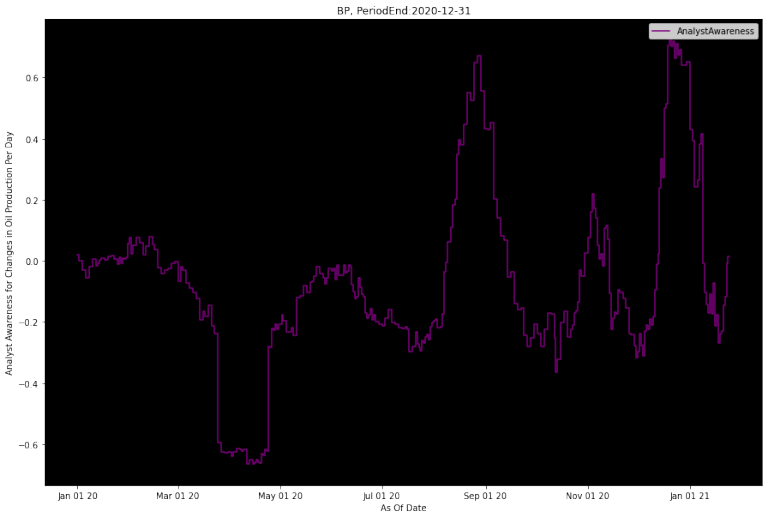
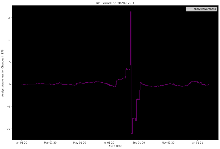
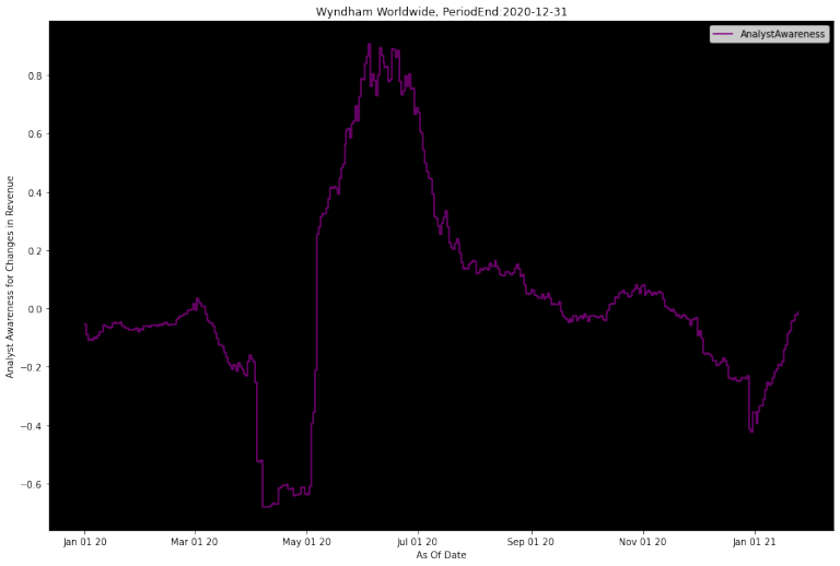
Analyst Awareness is something we came up with during our research process. We wanted to create a signal that would summarize whether analysts were aware of whatever was motivating the company to make changes in job postings. It should usually be close to zero, but when it deviates far away, that indicates a signifciant job posting change occured, but analysts have not revised accordingly.
In the example below, you'll see in March/April how the Analyst Awareness metric gets strongly negative when a lot of job postings are removed. This is preceding an eventual revision downwards by analysts. Similarly, it is strongly positive coming into September, when there is an increase in job postings before analysts eventually revise up.
We've left the trailing lookback window as a parameter, setting it for 30-days in this example. Truth is our research priorities shifted and we never got to dive deeper into this to find the optimal change window and refine the Analyst Awareness metric further. We hope that our initial research might inspire you to look at this further and maybe develop an extension of your own.
def chart_analyst_awareness(lookback_days, company_name, period_end, linkup_df, ibes_df, measure_name, plot_date_start, plot_date_end):
# Figure out the past date that will be used for trailing job calcuation
linkup_df['Date_past'] = linkup_df['Date_'] - pd.to_timedelta(lookback_days, unit='d')
# Self-join the dataframes, offset by the trailing window
linkup_trailing_df = linkup_df.merge(linkup_df, left_on='Date_past', right_on='Date_', suffixes=('_present', '_past'))
# Calculate the change over the trailing window
linkup_trailing_df['trailing_job_chg'] = (linkup_trailing_df['UniqueActiveJobCount_present'] - linkup_trailing_df['UniqueActiveJobCount_past']) / linkup_trailing_df['UniqueActiveJobCount_past']
# Create a daily time series for all the days you want to populate
daily_dates = pd.DataFrame({'EffectiveDate':pd.date_range(ibes_df['EffectiveDate'].min(), plot_date_end, freq='D')})
# Create a date-type from datetime, for easier merging
daily_dates['AsOfDate'] = pd.to_datetime(daily_dates['EffectiveDate']).dt.date
ibes_df['AsOfDate'] = pd.to_datetime(ibes_df['EffectiveDate']).dt.date
# Daily-ized I/B/E/S Estimates, carrying forward the estimates
daily_ibes_df = daily_dates.merge(ibes_df, how='left', on='AsOfDate').ffill()
# Figure out the past date that will be used for trailing job calcuation
daily_ibes_df['AsOfDate_past'] = daily_ibes_df['AsOfDate'] - pd.to_timedelta(lookback_days, unit='d')
# Self-join the dataframes, offset by the trailing window
ibes_trailing_df = daily_ibes_df.merge(daily_ibes_df, left_on='AsOfDate_past', right_on='AsOfDate', suffixes=('_present', '_past'))
# Calculate the change over the trailing window
ibes_trailing_df['trailing_est_chg'] = (ibes_trailing_df['DefMeanEst_present'] - ibes_trailing_df['DefMeanEst_past']) / ibes_trailing_df['DefMeanEst_past']
# Now combine the LinkUp Jobs Chgs with the I/B/E/S Estimates changes
analyst_awarness_df = linkup_trailing_df.merge(ibes_trailing_df, left_on='Date__present', right_on='AsOfDate_present')
# Finally, create the Analyst Awareness metric
analyst_awarness_df['AnalystAwareness'] = analyst_awarness_df['trailing_job_chg'] - analyst_awarness_df['trailing_est_chg']
# Focus on recent times only
startdate = datetime.datetime.strptime(plot_date_start,'%Y-%m-%d').date()
enddate = datetime.datetime.strptime(plot_date_end,'%Y-%m-%d').date()
single_analyst_awareness = analyst_awarness_df[(analyst_awarness_df['Date__present']>=startdate) & (analyst_awarness_df['Date__present']<=enddate)]
chart_title = company_name + ", PeriodEnd:" + period_end
# Plot Analyst Awareness
aa_ax = single_analyst_awareness.plot(x='Date__present', y='AnalystAwareness', label='AnalystAwareness', drawstyle='steps-post', color='purple', figsize=(15,10), title=chart_title)
aa_ax.set_ylabel('Analyst Awareness for Changes in ' + measure_name)
# Some final formatting
aa_ax.xaxis.set_major_formatter(mdates.DateFormatter('%b %d %y'))
aa_ax.set_xlabel('As Of Date')
aa_ax.set_facecolor('Black')
chart_analyst_awareness(lookback_days, company_name, period_end, linkup_df, ibes_df, measure_name, plot_date_start, plot_date_end)
def chart_jobs_complete(orgpermid, measure, measure_name, period_end, period_type, plot_date_start, plot_date_end, lookback_days):
(companyid, company_name) = lookup_companyid(orgpermid, plot_date_start)
linkup_df = grab_linkup_data(companyid)
estimateid = lookup_estimateid(orgpermid, plot_date_start)
ibes_df = grab_ibes_data(estimateid, measure, period_end, period_type)
se_df = grab_se_data(estimateid, measure, period_end, period_type)
chart_jobs(company_name, period_end, linkup_df, ibes_df, se_df, measure_name, plot_date_start, plot_date_end)
chart_analyst_awareness(lookback_days, company_name, period_end, linkup_df, ibes_df, measure_name, plot_date_start, plot_date_end)
EPS estimates
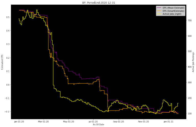
Initially, you'll notice a slight Active Job Postings decrease before EPS revisions. But later on the Active Job Postings drop significantly well before EPS estimates are revised down.
Also, notice how StarMine SmartEstimates revise down a little before the I/B/E/S Mean Consensus Estimates, that's because SmartEstimates given more weight to the higher rated analysts.
chart_jobs_complete(orgpermid, 9, "EPS", period_end, period_type, plot_date_start, plot_date_end, lookback_days)
Look at Revenue estimates
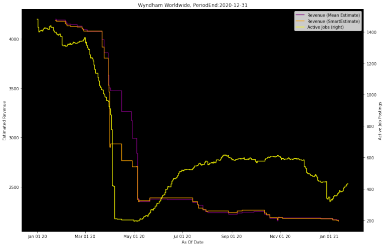
Now let's look at a different metric, Revenue, for a different company, Wyndham Worldwide, in a completely different industry. A quick switch up like this is easy since everything is parameterized in the chart_jobs_complete function.
Here we see active job postings dip in March/April well before the I/B/E/S consensus estimate revises down. The Analyst Awareness metric highlights this as well with a big dip around the same time. It's also worth noting that the SmartEstimate was slightly ahead of the I/B/E/S consensus estimate revision, until they eventually converged in May.
You'll also notice that active job postings have been steadily increasing since that dip, but analysts never revised upwards. Even coming into 2021, there is another increase in active job postings. However, neither active job postings bursts are anywhere near pre-pandemic levels. It's hard to come to a conclusion by looking at LinkUp Active Jobs or the Analyst Awareness metric alone here, but a situation like this might warrant a closer look by human investors covering this company.
chart_jobs_complete(4295916199, 20, "Revenue", '2020-12-31', period_type, plot_date_start, plot_date_end, lookback_days)
Conclusion
In conclusion, looking (as an example) at BP, we can see that one may be able to use LinkUp's Job Postings Data in Refinitiv Quantitative Analytics to foresee changes in KPIs from I/B/E/S or Smart Estimate changes via a graphical analysis. More research would be needed to see if such an analysis is sufficient in foreseeing changes in revenues or for other companies. One may use the insight following from the investigations above as a start and potentially then try to go through more empirical methods to determine the underlying mechanics and correlations at play, potentially with more complex methods (e.g.: involving machine learning or econometric methods).
References
The below documentation will be helpful should you wish to dive in further.