


Introduction
The official US crude exports figures are available from U.S. Energy Information Administration (EIA). However, these figures are published with a 2-3 months delay. In the world of alternative data sources, could we reliably estimate U.S. crude exports ahead of the official figures? In this example we're using trade flows data retrieved using LDMS (LSEG Data Management Solution) to gain insight into crude oil supply trends and buying patterns.
Retrieving trade flow data from LDMS and estimating U.S. crude exports.
LDMS is an open platform that allows you to integrate the great depth and breadth of LSEG’s commodity data into your workflows. LDMS merges and normalizes data across a range of sources including LSEG, 3rd party and internal customer's data. LSEG sources available through LDMS include our Real-Time datafeed, DataScope Select and Pointconnect feeds. Client application can conveniently retrieve this data using a standard REST API.
We start by retrieving the data for Dirty flows with Load Country as USA/Virgin Islands and Crude Oil as the Product. We also load Canada pipeline imports data, which we will later add to tanker crude flows originating from U.S. ports to estimate total U.S. crude exports. Static CSV file with U.S. ports locations is used to display port locations on the map.
#A config file with the LDMS api key is stored and accessed separately
config = configparser.ConfigParser()
config.read('config.ini')
api=config['LDMS']['Api']
headers = { 'Authorization' : config['LDMS']['Key'],'Accept':"text/csv" }
#params
flowType = 'Dirty'
fields = '*'
filter = 'LoadCountry=United States,Virgin Islands (U.S.);Product=Crude Oil'
result = requests.get(api + '/Flows/FlowData/'+flowType+'?Fields='+fields+'&Filter='+filter, headers=headers, verify=True)
flows = open('USflows.csv', "w")
flows.write(result.text)
flows.close()
df=pd.read_csv('USflows.csv', parse_dates=True, infer_datetime_format=True)
port_locations=pd.read_csv("US_Ports_Locations.csv")
canada_imports=pd.read_csv("Canada Pipeline Imports.csv",parse_dates=True,index_col='Bbls',thousands=',')
canada_imports.index=canada_imports.index.to_period('M')
#Display a sample of flows data we'll be analizing
df[['Departure Date','Vessel','Vessel Type','Load Port','Discharge Port','Barrels','Status']].tail(10)
Here's a sample of the flows data we're going to analyze.
| Departure Date | Vessel | Vessel Type | Load Port | Discharge Port | Barrels | Status |
| 5/16/21 11:40 | SOCRATES | Panamax | Beaumont | NaN | 483,835 | Vessel Underway |
| 5/16/21 18:15 | EAGLE HELSINKI | Aframax / LRII | GOLA - Galveston Offshore Lightering Area | Corpus Christi | 413,072 | Vessel Underway |
| 5/18/21 12:00 | PEGASUS VOYAGER | Suezmax | Pacific Area Lightering | NaN | 951,663 | Vessel Loading |
| 5/18/21 12:00 | OLYMPIC LION | VLCC | Corpus Christi | NaN | 1,998,133 | Vessel Loading |
As we can see from this sample, on May 16, 2021 an Aframax class vessel named Eagle Helsinki was carrying 413 thousand barrels of oil from Galveston Offshore Lightering Area to Corpus Christi, and a VLCC named Olympic Lion was being loaded with almost 2 mln barrels of oil at Corpus Christi for departure on May 18, 2021.
To produce an estimate for monthly crude exports we need to aggregate the flows into time intervals. For this purpose it's useful to add a number of columns detailing departure and arrival week, month, quarter and year.
df['DepartureDate'] = pd.to_datetime(df['DepartureDate'], errors='coerce')
df['ArrivalDate'] = pd.to_datetime(df['ArrivalDate'], errors='coerce')
df['Departure Week Number']=df['DepartureDate'].dt.week
df['Departure Week']=pd.to_datetime(df['DepartureDate']).dt.to_period('w')
df['Departure Month']=pd.to_datetime(df['DepartureDate']).dt.to_period('M')
df['Departure Quarter']=pd.to_datetime(df['DepartureDate']).dt.to_period('Q')
df['Departure Year']=pd.to_datetime(df['DepartureDate']).dt.to_period('Y')
df['Arrival Week Number']=df['ArrivalDate'].dt.week
df['Arrival Week']=pd.to_datetime(df['ArrivalDate']).dt.to_period('w')
df['Arrival Month']=pd.to_datetime(df['ArrivalDate']).dt.to_period('M')
df['Arrival Quarter']=pd.to_datetime(df['ArrivalDate']).dt.to_period('Q')
df['Arrival Year']=pd.to_datetime(df['ArrivalDate']).dt.to_period('Y')
Now we analyze the flows by geography.
Myanmar discharges are treated as imports by China as the Sino-Myanmar pipeline feeds the refineries in China provinces bordering Myanmar.
The trade flows data includes all crude transport. At the moment there's only one U.S. facility (The Louisiana Offshore Oil Port or LOOP) able to accommodate a fully loaded VLCC (Very Large Crude Carrier), a type of oil tanker able to carry approximately 2 mln barrels of crude oil and required for economic transportation of crude across the ocean, such as between the U.S. and Asia. All onshore U.S. ports in the Gulf Coast that actively trade petroleum are located in inland harbors and are connected to the open ocean through shipping channels or navigable rivers. Although these channels and rivers are regularly dredged to maintain depth and enable safe navigation for most ships, they are not deep enough for deep-draft vessels such as fully loaded VLCCs. To circumvent depth restrictions, VLCCs transporting crude oil to or from the U.S. Gulf Coast have typically used partial loadings and the process of ship-to-ship transfers or lightering. To accurately estimate U.S. crude exports, we need to account for lightering in our analysis of trade flows data, to avoid double counting crude first transported in a smaller tanker from a U.S. onshore port to an offshore lightering zone and then transferred to a larger tanker for trasporting to its ultimate destination port.
Flows are segregated based on their load and discharge port/berth characteristics to avoid double counting of ship-to-ship (STS) loads. Only STS loads with discharge country other than US/Virgin Islands and shore loads with discharge country other than US/Virgin Islands are counted towards exports. Vessels with status as Underway, Discharged, Discharging or Awaiting Discharge are departed flows and are included in the count.
df['Adjusted Discharge Country']=np.where(df['Discharge Country']=='Myanmar','China',df['Discharge Country'])
sts_port_exclusion_list=['C}TS7309641681','C}TS7309533579','C}TS7309533561','C}TS7309786001','C}TS7309709063','C}TS7309557398',
'C}TS7309789693','C}TS7309823983','C}TS7309564485','C}TS7309533587','C}TS7309791374','C}TS7309944668']
df['Loadport_exclusion']=np.where(df['Load Port RIC'].isin(sts_port_exclusion_list),1,0)
df['Disport_exclusion']=np.where(df['Load Port RIC'].isin(sts_port_exclusion_list),1,0)
df['Discharge_country']=np.where(df['Discharge Country'].isin(['United States','Virgin Islands (U.S.)']),1,0)
df['Flow_exclusion']=np.where((df['Discharge_country']==0)&(df['Loadport_exclusion']==0),1,
np.where((df['Discharge_country']==0)&(df['Loadport_exclusion']==1),1,0))
us_exports=df[df['Flow_exclusion']==1]
us_exports=us_exports[us_exports['Status'].isin(['Vessel Underway','Vessel Discharged','Vessel Discharging','Vessel Awaiting Discharge'])]
zones=pd.read_csv("ports_zones.csv")
merged_df=us_exports.merge(zones,how='left',left_on='Load Port RIC',right_on='Ric')
merged_df=merged_df.merge(port_locations,how='left',left_on='Load Port RIC',right_on='Instrument')
In the code snippet above we added port zone info to the dataframe. This allows us to demonstrate that trade flows analysis can be done for a specific PADD. In this example we're only going to consider PADD 3 exports, which account for the bulk of U.S. crude exports. To achieve this, we're filtering flows with Tanker zone as US Gulf. Then we can pivot the table to aggregate the flow by departure month and add Canada imports via pipelines.
padd3=merged_df[merged_df['Tanker Zone']=='US Gulf']
padd3_table=padd3.pivot_table(index='Departure Month',values='Barrels',aggfunc=np.sum,fill_value=0)
padd3_table=padd3_table.merge(canada_imports['PADD 3'],how='left',left_index=True,right_index=True)
padd3_mnbpd=padd3_table.copy()
padd3_mnbpd['days']=np.where(padd3_mnbpd.index!=pd.Timestamp(dt.datetime.today()).to_period('M'),padd3_mnbpd.index.days_in_month,dt.datetime.today().day)
padd3_mnbpd['mnbpd']=padd3_mnbpd.iloc[:,0]/(padd3_mnbpd['days'])
padd3_mnbpd['LSEG Flows_kbpd']=padd3_mnbpd['mnbpd']/1000
padd3_mnbpd['Pipeline exports_kbpd']=padd3_mnbpd['PADD 3']/1000/(padd3_mnbpd['days'])
padd3_mnbpd.drop(columns='days',inplace=True)
print(padd3_mnbpd.tail())
To visualize how well our estimated PADD 3 exports compare to the official figures from EIA, we're using the Data Library to retrieve the timeseries of EIA U.S. PADD 3 crude oil exports, construct a comparison table and plot the timeseries.
eia=ld.get_history('EXP-CLPD3D-EIA',start='2015-01-01', end='2025-05-30', interval='monthly')
eia.index=eia.index.to_period('M')
compare=padd3_mnbpd.merge(eia,how='left',left_index=True,right_index=True)
compare['PADD3_calculated']=compare['LSEG Flows_kbpd']+compare['Pipeline exports_kbpd']
compare.index=compare.index.astype('str')
compare['COMM_LAST']=compare['COMM_LAST'].astype('float64')
fig_benchmarking=compare[['LSEG Flows_kbpd','Pipeline exports_kbpd']].iplot(kind='bar',barmode='stack',title='Comparison of EIA and LSEG Oil Research flows for US PADD 3 Crude Oil exports',asFigure=True)
fig_benchmarking.add_trace(trace=go.Scatter(x=compare.index,y=compare['COMM_LAST'],name='EIA PADD3',line=dict(color='lime')))
fig_benchmarking.show()
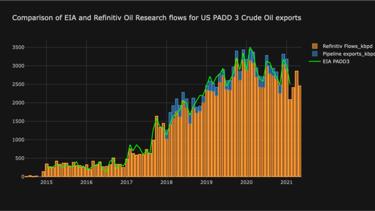
As one can clearly see from the chart, LSEG Flows data for seaborne exports historically tracks the official EIA figures with very high degree of accuracy. The advantage of our estimate over official EIA data is of course that our estimate can be performed in real-time.
Using Fixtures data to forecast crude exports.
Finally we're going to see if fixtures data could be a predictor of U.S. crude exports. We retrieve LSEG Fixtures data through LDMS API call and combining it with our estimates of crude exports from PADD 3 we compiled before using trade flows.
fixturesType = 'Tanker'
fields = '*'
headers = { 'Authorization' : config['LDMS']['Key'],'Accept':"text/csv" }
result = requests.get(api + '/Fixtures/FixtureData/'+fixturesType+'?Fields='+fields, headers=headers, verify=True)
fixtures = open('Fixtures.csv', "w")
fixtures.write(result.text)
fixtures.close()
fixtures_df=pd.read_csv('Fixtures.csv',parse_dates=True,infer_datetime_format=True, encoding='latin-1')
filtered_fixtures_df=fixtures_df[fixtures_df['Load Zone']=='US Gulf']
filtered_fixtures_df=filtered_fixtures_df[filtered_fixtures_df['Commodity']=='Crude Oil']
filtered_fixtures_df['Laycan Month']=pd.to_datetime(filtered_fixtures_df['Laycan From']).dt.to_period('M')
fix_pivot=filtered_fixtures_df.pivot_table(index='Laycan Month',values='Cargo Size',aggfunc=np.sum)
fix_pivot=fix_pivot.merge(padd3_mnbpd,how='left',left_index=True,right_index=True)
fix_pivot.drop(columns=['PADD 3','mnbpd','Pipeline exports_kbpd'],inplace=True)
fix_pivot['Cargo Size']=fix_pivot['Cargo Size']*7.3 #Converting from Tonnes to Barrels using BPT
fix_pivot=fix_pivot.loc[pd.Period('2020-01'):]
fix_pivot.index=fix_pivot.index.astype('str')
fig_fix=fix_pivot[['Barrels']].iplot(kind='bar',title='PADD 3 exports vs Fixtures',asFigure=True)
fig_fix.add_trace(trace=go.Scatter(x=fix_pivot.index,y=fix_pivot['Cargo Size'],name='Fixtures qty',line=dict(color='lime')))
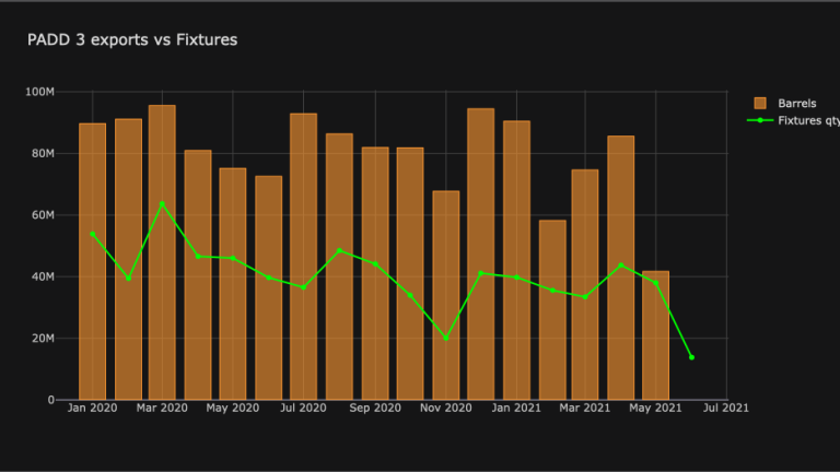
What we can see from this chart is that LSEG Fixtures show good correlation with estimated crude exports from PADD 3, and can be reasonably used as a predictor of the direction or trend of U.S. crude exports. Similar analysis can be done for other regions or commodities.
Complete source code for this article can be downloaded from Github