Delta Hedging - Simplify your Option Pricing

In this article, I will demonstrate workflows used to manage risk, specifically focusing on the most widely used Greek (Delta), as a tool to hedge common strategies.

Development Tools & Resources

The example code demonstrating the use cases are based on the following development tools and resources:

• Refinitiv Data Platform (RDP): Access to the platforms pricing endpoint data services

• Python Environment:
  • Tested with Python 3.7
  • Packages: refinitiv.dataplatform pandas json datetime math dateutil enum
  • RDP for Python installation: pip install refinitiv-dataplatform

• .NET Environment:
  • Tested with .Net Core 3 (Visual Studio 2019)
  • NuGet: Refinitiv.DataPlatform.Content
  • RDP for .NET installation: Installed as part of the example package within Visual Studio

Overview

Working through some of the common strategies and workflows when managing your risk, you are typically required to utilize some critical resources to simplify the effort. For example, the ability to retrieve market data metrics, accessing option chains to select your positions, calculators to price your Volatility Curves and Greeks, etc. By utilizing Instrument Pricing Analytics (IPA) and market data pricing services from Refinitiv, the workflows presented will demonstrate the algorithms used to provide these critical resources as the basis for our strategies. The intention here is to not only demonstrate value-add workflows but to also showcase the capabilities of the pricing analytics to provide the reader with the tools to model their strategies to manage risk.

Use Cases

Each use case below will outline the basics of building out the strategies using the Options Price Contracts interface. To explain the basics for each strategy, I will be using two different modeling features defining the delta metric. The interface supports both ETI (Exchange-Traded-Instruments) as well as OTC (Over-The-Counter) pricing models to allow us to showcase both interfaces to drive our specific use case.

Use Case 1 - Long Strangle

The Long Strangle is a strategy that profits when you expect a big move in the underlying stock. The strategy typically involves buying both a Put and Call out-of-the-money with the same expiration date.  The goal of the strategy is to profit from a substantial movement in the price of the stock sometime in the future.   The choice of the asset as well as the anticipated expiry of the price movement is key to the success of the strategy.

While we know delta is a measurement of an option's price sensitivity to a given change in the price of an underlying asset, many traders think of delta as the percent probability of being in the money. In this strategy, I would like to construct a long strangle that has a ~70% chance of being in the money, according to delta. To accomplish this, I'm going to use a delta that has an approximately 35% probability of being in the money, for each leg (Call and Put) of my strangle.

The strategy will demonstrate a workflow that presents an option chain to choose the appropriate legs making up our strangle. The following steps will be used:

1. Query and present an option chain containing our legs
2. Demonstrate the strategy by choosing the appropriate legs and build out a profit model

Building an option chain

An option chain can contain up to thousands of contracts, spanning multiple years, defining both call and put contracts at different price levels. When building the strangle strategy, 2 legs with the same expiry must be chosen. The algorithm provided allows the user to narrow down our option chain by selecting a specific expiry and a strike that is a certain percentage around-the-money. This will allow users to fine-tune these input parameters to present a suitable option chain to select the appropriate legs to build out the strategy.

We first define our data endpoint then issue the call to request for the complete list of constituents making up the chain:

Each constituent within our chain is comprised of a root, the details of the expiration, and the strike price. As we iterate through the complete chain, we apply the filter and decide which constituents we want to keep. For each filtered constituent, we'll store within either a Call or Put collection list.

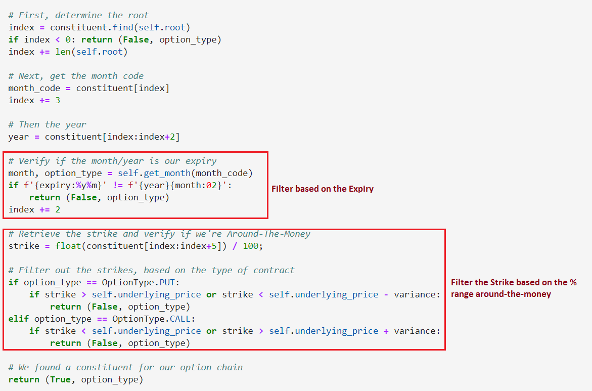
Our filter method keep_constituent() breaks down the constituent into individual parts for us to determine whether we want to keep it, based on our input filter parameters:

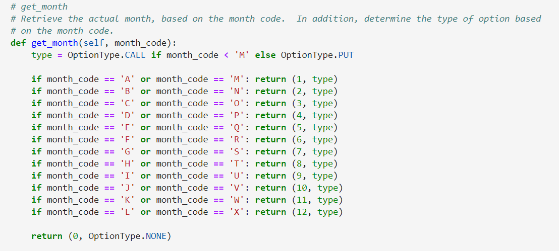
You can see the 2 main code sections that filter out based on the expiry and whether the strike is around-the-money. Also, we can determine whether the option is a Call or Put, based on the contract month code.

We use the option type to determine which collection to file the constituent.

Finally, we combine our Call and Put collections into an option chain:

Based on my get_contracts() request, the following option chain retrieved 23 contracts.

With these contracts, we can now move on to step #2 and feed this collection into our Analytics engine to price our options:

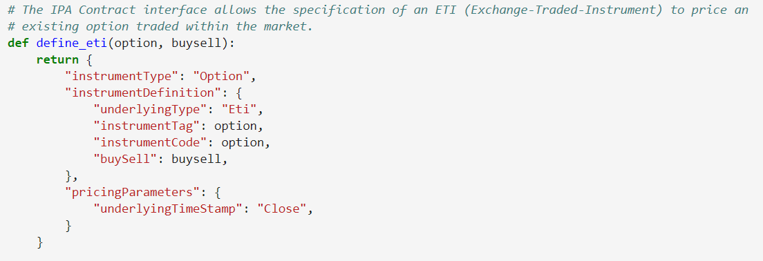
The Analytics engine provides the ability to price Exchange Traded Instruments via the IPAOption class. The class utilizes the Financial Contracts endpoint defined within IPA as the main interface to model my use cases.

The following code segment is used to price our ETI option contracts:

To model an ETI Option, the analytics engine requires the Options RIC (instrumentCode) and whether we are buying or selling as the basis to price the option details. The engine will be responsible for doing all the heavy lifting of determining the underlying RIC and its price, as well as the details of the option such as the strike price, expiry date, and whether it is a Put or Call option. The engine will then use the necessary algorithms to price the Greeks, specifically delta in our examples.

To price our contracts, we issue the following code segment to the platform:

The IPA Option interface provides the ability to submit many request parameters down to the Analytics engine and compute the desired values, such as delta. While the purpose of this article is to compute delta, a number of other underlying properties are also determined which will help piece together the different strategies.

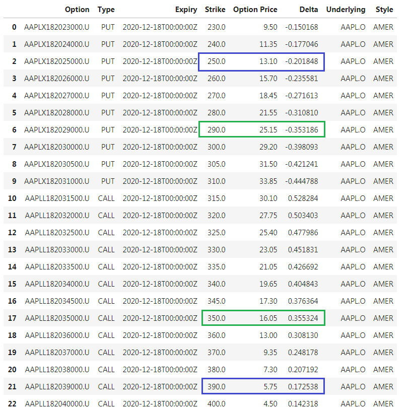
Once submitted, the resulting option chain containing our pricing details is presented:

As you can see, all contracts have the same December 2020 expiry. To construct the long strangle, I referred to the Call and Put contracts above to represent my legs in the strategy, specifically choosing contracts that have deltas at or near .35.

With Apple trading at $314.96, I've chosen to select the 290 put and 350 call (in green) as my legs. With these two legs, they collectively provide a strategy that is roughly 70% probability of being in the money. While this can provide the basis of my strategy, it is important to consider the cost of the transaction, i.e. the premiums paid for each leg.

The total cost of the trade:

To see a profit (not including fees and commissions), the break-even above the current market price ($314.96) is:

And the break-even below the current market price is:

If we look at strike prices (in blue) based on the above break-even values, we can approximate the probability of profit as:

A trader would utilize this strategy in anticipation there is expected to be a substantial movement in the price of the stock until expiration. However, there is the consideration to sell a long strangle as you may anticipate there will not be a lot of volatility. Using the above example, shorting the strangle would have a ~30% of success. Using the same logic above you can refer to the option chain and choose deltas around 0.15 and build the model from there to determine the probability of profit.

Use Case 2 - Delta Neutral

Delta Neutral is a strategy utilizing multiple positions that aim to provide an overall delta totaling zero. When an initial position is taken at a given point in time, the strategy involves reacting to changes in the market by buying or selling assets such that positive and negative deltas total to or near zero. Within this use case, using the option IPA interfaces, I will model scenarios to demonstrate how the value of delta is affected by market changes. Specifically, I can model scenarios such as changes in the underlying price or the effect as the time approaches maturity and how I can respond to these changes by buying or selling option positions to maintain a neutral strategy.

Let's assume I'm taking an initial position where I'm long 500 shares of Apple stock.

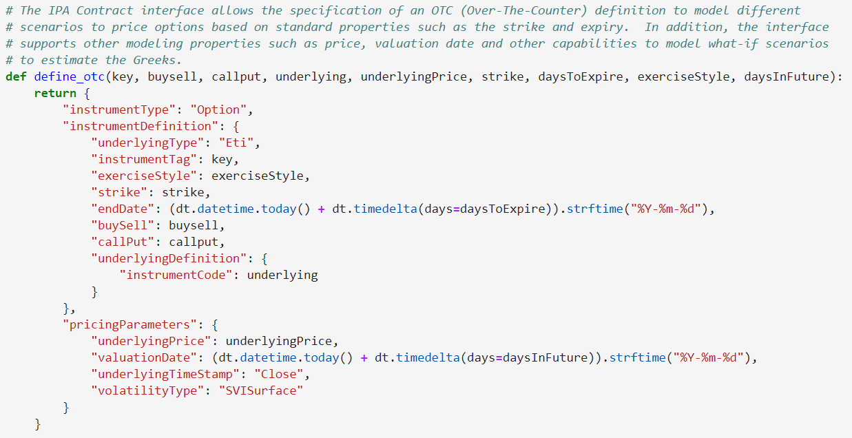
The DeltaNeutral class allows me to define an initial position. Using the same IPAOption class defined in Use Case 1, I instead utilize the OTC capabilities within the Analytics engine:

To model an OTC Option, the analytics engine requires not only the Options RIC (instrumentCode), but details such as the strike, expiry, and whether it is a Put or Call option. While the engine can compute the underlying price to help model the Greeks, I've chosen to set my price (underlyingPrice) instead of the engine figuring it for me. This allows me to compute what the delta would look like when the price changes. Also, I can choose a valuation date that allows me to predict what the calculations look like N months from now. The goal is to model different scenarios based on possible outcomes in the market. With OTC modeling, there is no quoted option so the engine computes the Volatility Surface to simulate or predict the implied volatility used to drive the calculations within the engine.

In an attempt to hedge my initial position, I decided to model a scenario where I plan to short some Call Options. By utilizing the capabilities of IPA to model my own OTC position, I decided to write a Call using a strike of 7.5% out-of-the-money with an expiry about 1 year from today. I can acquire the delta which shows my current portfolio:

The update_portfolio() method determines how many contracts I need to write to put me as close as possible to delta-neutral. As you can see, by selling 12 Call Options, puts me in a net delta position of 18.

However, as time passes and as market conditions change, the net delta position of the portfolio will change. For example, once again using some additional capabilities of the IPA engine, I can create a scenario to see what my net delta position will look like 60 days from now. With this, I'm going to assume the price of the underlying has increased by 5%:

As market conditions change, the value of delta has changed and thus the overall net position of my portfolio has changed. At this point, I have many choices from either selling some of my long position or perhaps introducing a new position in an attempt to hedge the strategy.

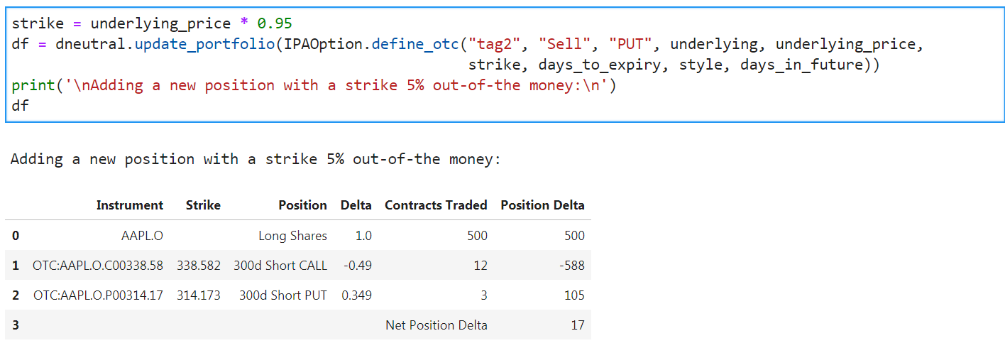
For example, I decided that I may want to short some Put Options with a strike 5% out-of-the-money:

Based on the delta, to balance my portfolio, I must sell 3 Put Options to bring me reasonably close to delta-neutral.

The algorithms presented here coupled with the simplicity of the Analytics engine provide several different what-if scenarios to build our strategy. Traders can predict or model different scenarios, using simulated market conditions.

Closing Summary

The above use cases were selected to showcase some of the capabilities of the IPA interfaces. Also, by utilizing the chain interfaces within the platform, I can easily filter-down the list of contracts that make up my option chain in order to effectively choose the legs of the strangle outlined in the first use case. While the focus of the article was around delta, many strategies are built around other key Greek measures which can easily be obtained using the techniques presented here. As you can imagine, there several strategies and modeling scenarios that can be applied by using the capabilities within the platform.

Further Readings

Discover our new upcoming Refinitiv Data Platform Library - Part 1 of my RDP Library Introduction article

Q&A Forum for the Refinitiv Data Platform Library