Author:

Jirapongse Phuriphanvichai
Developer Advocate
Developer Advocate
Updated: 05 Mar 2025
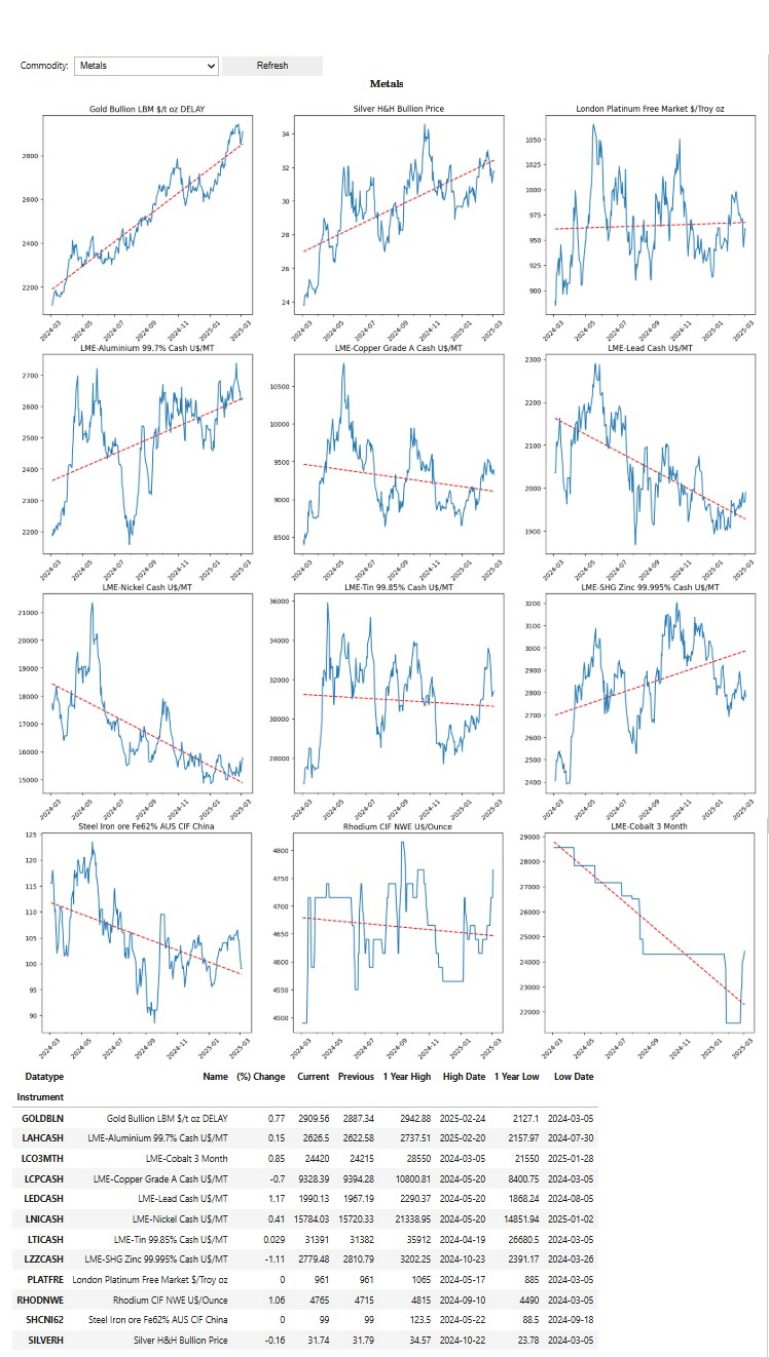
The Datastream Commodities Overview illustrates recent price movements for key commodities in the Metals, Energy, Chemicals, Agriculture, and Indices. It uses DataStream Web Services to retrieve the one-year historical price for commodities and then plot line charts with trend lines that demonstrate directions and movements of prices. It also shows summary data such as, percentage change, one year low, and one year high in the table. It is similar to the Datastream Commodities Overview in the LSEG Workspace Excel Template Library.
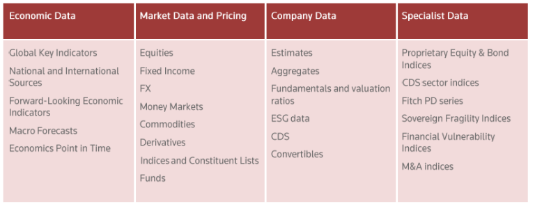
Datastream
Datastream is the world’s leading time-series database, enabling strategists, economists, and research communities’ access to the most comprehensive financial information available. With histories back to the 1950s, you can explore relationships between data series; perform correlation analysis, test investment and trading ideas, and research countries, regions, and industries.
The Datastream database has over 35 million individual instruments or indicators across major asset classes. You can directly invoke the web service methods from your applications by using the metadata information we publish.
The Datastream Web Service allows direct access to historical financial time series content listed below.
For more information, please refer to Datastream Web Service.
DatastreamPy
This example uses the DatastreamPy library to connect and retrieve data from Datastream. To use this Python library, please refer to the Getting Started with Python document.
Loading Libraries
The required packages for this example are:
- DataStreamPy: Python API package for Datastream Webservice
- matplotlib: A comprehensive library for creating static, animated, and interactive visualizations in Python
- pandas: Powerful data structures for data analysis, time series, and statistics
- dateutil: Powerful extensions to the standard datetime module
- ipywidgets: IPython HTML widgets for Jupyter
- numpy: The fundamental package for array computing with Python
import numpy as np
import matplotlib.pyplot as plt
import dateutil
import matplotlib.dates as mdates
import DatastreamPy as DSWS
import pandas as pd
import ipywidgets as widgets
from ipywidgets import Button, HBox, VBox, Dropdown, Label, Layout
Setting Credentials
The DataStream username and password are required to run the example.
ds = DSWS.DataClient(None, username = '<username>', password = '<password>')
Specifying Data Types and Expressions
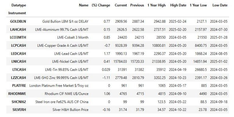
The following fields are displayed in the summary table.
| Data Types or Expressions | Descriptions |
|---|---|
| NAME | The name of the equity/company or equity list, as stored on Datastream’s databases |
| PCH#(X,-1D) | The percent change percent from yesterday to today |
| X | Today's price| |
| VAL#(X,-1D) | Yesterday's price| |
| MAX#(X,-1Y) | The highest price within one year |
| MAXD#(X,-1Y) | The date of the highest price| |
| MIN#(X,-1Y) | The lowest price within one year |
| MIND#(X,-1Y) | |The date of the lowest price |
The variable is specified as a class. The keys contain the data types or expressions and the values contain descriptions.
You can access the Datastream Navigator to search for data types or instruments. For other expressions, refer to the Datastream help page.
summary_fields = {
'NAME':'Name',
'PCH#(X,-1D)':'(%) Change',
'X':'Current',
'VAL#(X,-1D)':'Previous',
'MAX#(X,-1Y)':'1 Year High',
'MAXD#(X,-1Y)':'High Date',
'MIN#(X,-1Y)':'1 Year Low',
'MIND#(X,-1Y)':'Low Date'
}
Specifying Instruments
Next, I specify instruments of key commodities in the Metals, Energy, Chemicals, Agriculture, and Indices.
Metals
| Instruments | Descriptions |
|---|---|
| GOLDBLN | Gold Bullion LBM $/t oz DELAY |
| SILVERH | Silver, Handy&Harman (NY) U$/Troy OZ |
| PLATFRE | London Platinum Free Market $/Troy oz |
| LAHCASH | LME-Aluminium 99.7% Cash U$/MT |
| LCPCASH | LME-Copper Grade A Cash U$/MT |
| LEDCASH | LME-Lead Cash U$/MT |
| LNICASH | LME-Nickel Cash U$/MT |
| LTICASH | LME-Tin 99.85% Cash U$/MT |
| LZZCASH | LME-SHG Zinc 99.995% Cash U$/MT |
| SHCNI62 | Steel Iron ore Fe62% AUS CIF China |
| RHODNWE | Rhodium CIF NWE U$/Ounce |
| LCO3MTH | LME-Cobalt 3 Month |
Energy
| Instruments | Descriptions |
| OILBREN | Crude Oil BFO M1 Europe FOB $/BBl |
| OILWTXI | Crude Oil WTI NYMEX Close M U$/BBL |
| GASUREG | Gasoline,Unld. Reg. Oxy. NY Cts/Gal |
| DIESELA | Diesel, .05% Sulphur LA C/GAL |
| NATGAS1 | NYMEX Natural Gas Henry Hub C1 |
| FUELOIL | Fuel Oil No.2 (New York) C/Gallon |
| LGOLCO1 | GasOil/Brent Crude Spread U$ |
| OILMCPC | Crude Oil MED Urals 140kt CIF U$/BBL |
| NATBGAS | ICE Natural Gas 1 Mth.Fwd. P/Therm |
| LMCYSPT | Coal ICE API2 CIF ARA Nr Mth $/MT |
| EEXPEAK | EEX - Phelix Peak Hr.09-20 E/Mwh |
| POWBASE | Powernext Elec. Baseload E/Mwh |
Chemicals
| Instruments | Descriptions |
|---|---|
| PFPENPU | LDPE FD Europe Spot NWE E/MT |
| OLETFPU | Ethylene FD European NWE E/MT |
| PFPCOPU | PP Copolymer Europe Cont German E/MT |
| ARSXRPU | PVC,USG Domestic GP UC/LB |
| CUTNMET | Titanium Dioxide EXW R-996 Tax Inclu |
| OLBURPU | Butadiene Europe Rdam FOB $/MT |
| ETHANYH | Expandab Polystyrene FDC UK £/MT |
| STEPUPU | Polystyrene-GP, Dom FD UK £/MT |
| VPVCUPU | PVC Suspension US FAS Houston $/M |
| ARPXKPU | Paraxylenes Korea FOB U$/MT |
| INMCNPU | Monoethylene Glycol CFR China $/MT |
| ARBNUPU | Benzene US Gulf FOB USc/GAL |
Agriculture
| Instruments | Descriptions |
|---|---|
| WHEATSF | Wheat No.2,Soft Red U$/Bu |
| CORNUS2 | Corn No.2 Yellow U$/Bushel |
| RIT1STA | Rice, White 100% FOB Bangkok U$/MT |
| WOLAWCE | Wool AWEX E.M.I. A$/100KG |
| WSUGDLY | Raw Sugar-ISA Daily Price c/lb |
| COCINUS | Cocoa-ICCO Daily Price US$/MT |
| COTTONM | Cotton,1 1/16Str Low -Midl,Memph $/Lb |
| SOYBEAN | Soyabeans, No.1 Yellow $/Bushel |
| PAOLMAL | Palm Kernel Oil MAL CIF Rdam US$ /MT |
| CLHINDX | CME - Lean Hog Index |
| USTEERS | Live Steers, USDA 5 Area Wtd. Avge. |
| MILKGDA | CME-Milk Non Fat Dry Grade A Spot |
Commodities Indices
| Instruments | Descriptions |
|---|---|
| GSCITOT | S&P GSCI Commodity Total Return |
| DJUBSTR | Bloomberg- Commodity TR |
| RICIXTR | Rogers International Commodity Ind TR |
| RJEFCRT | RF/CC CRB TR |
| MLCXTOT | MLCX Total Return |
| DBKLCIX | DBLCI Optimum Yield Diversifi ER Idx |
| BALTICF | Baltic Exchange Dry Index (BDI) |
| LMEINDX | LME-LMEX Index |
| DRAMDXI | DRAMeXchange-DXI Index |
| GSGCTOT | S&P GSCI Gold Total Return |
| SPGCHPG | GSCI Gasoline |
| SGPDTOT | S&P GSCI Palladium Index TR |
All instruments and summary fields are set into the commodities variable with categories as key names.
{'Metals': {'Items': ['GOLDBLN', 'SILVERH', ...], 'Fields': {'NAME': 'Name', 'PCH#(X,-1D)': '(%) Change', ...}}, 'Energy': {'Items': ['OILBREN', 'OILWTXI', ...], 'Fields': {'NAME': 'Name', 'PCH#(X,-1D)': '(%) Change', ...}}, 'Chemicals': {'Items': ['ETYEUSP', 'PPPEUSF', ...], 'Fields': {'NAME': 'Name', 'PCH#(X,-1D)': '(%) Change', ...}}, 'Argiculture': {'Items': ['WHEATSF', 'CORNUS2', ...], 'Fields': {'NAME': 'Name', 'PCH#(X,-1D)': '(%) Change', ...}}, 'Indices': {'Items': ['GSCITOT', 'DJUBSTR', ...], 'Fields': {'NAME': 'Name', 'PCH#(X,-1D)': '(%) Change', ...}}} |
commodities = {}
# Metals
commodities['Metals'] = {}
commodities['Metals']['Items']=[
'GOLDBLN','SILVERH','PLATFRE','LAHCASH',
'LCPCASH','LEDCASH','LNICASH','LTICASH',
'LZZCASH','SHCNI62','RHODNWE','LCO3MTH']
commodities['Metals']['Fields']=summary_fields
# Energy
commodities['Energy'] = {}
commodities['Energy']['Items']=[
'OILBREN','OILWTXI', 'GASUREG','DIESELA',
'NATGAS1','FUELOIL','LGOLCO1','OILMCPC',
'NATBGAS','LMCYSPT','EEXPEAK','POWBASE']
commodities['Energy']['Fields']=summary_fields
# Chemicals
commodities['Chemicals'] = {}
commodities['Chemicals']['Items']=[
'PFPENPU','OLETFPU','PFPCOPU','ARSXRPU',
'CUTNMET','OLBURPU','ETHANYH','STEPUPU',
'VPVCUPU','ARPXKPU','INMCNPU','ARBNUPU']
commodities['Chemicals']['Fields']=summary_fields
# Argiculural
commodities['Agriculture'] = {}
commodities['Agriculture']['Items']=[
'WHEATSF','CORNUS2','RIT1STA','WOLAWCE',
'WSUGDLY','COCINUS','COTTONM','SOYBEAN',
'PAOLMAL','CLHINDX','USTEERS','MILKGDA']
commodities['Agriculture']['Fields']=summary_fields
#Commodities Indices
commodities['Indices'] = {}
commodities['Indices']['Items']=[
'GSCITOT','DJUBSTR','RICIXTR',
'RJEFCRT','MLCXTOT','DBKLCIX',
'BALTICF','LMEINDX','DRAMDXI',
'GSGCTOT','SPGCHPG','SGPDTOT']
commodities['Indices']['Fields']=summary_fields
Defining a Widget to Display Commodities Overview
In this section, we will create a widget that displays Commodities Overview of a selected commodities' category (Metals, Energy, Chemicals, Agriculture, and Indices). After selecting the category, the widget uses the get_data method in the DataStreamPy library to retrieve daily historical prices for one year of the instruments in the selected category.
ds.get_data (tickers="GOLDBLN,SILVERH,PLATFRE,LAHCASH,
LCPCASH,LEDCASH,LNICASH,LTICASH,
LZZCASH,SHCNI62,RHODNWE,LCO3MTH", start='-1Y')
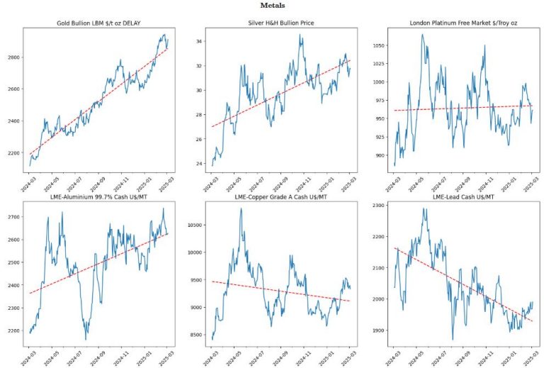
Then, it uses the matplotlib library to plot historical charts with trend lines of the returned prices.
Next, it calls the get_data method to retrieve the data for the summary fields and then displays the data in tabular format.
ds.get_data(tickers="GOLDBLN,SILVERH,PLATFRE,LAHCASH,
LCPCASH,LEDCASH,LNICASH,LTICASH,
LZZCASH,SHCNI62,RHODNWE,LCO3MTH",
fields=['NAME','PCH#(X,-1D)','X',
'VAL#(X,-1D)','MAX#(X,-1Y)','MAXD#(X,-1Y)',
'MIN#(X,-1Y)','MIND#(X,-1Y)'],
kind=0)
class CommodityOverviewWidget:
status_label = Label("")
cache = {}
title_label = Label(value='')
button = Button(description='Refresh')
output = widgets.Output()
commodity_dropdown = None
def __init__(self, _context):
dropdown_options = list(_context.keys())
self.commodity_dropdown = Dropdown(options=dropdown_options, value=dropdown_options[0],description='Commodity:')
display(HBox([self.commodity_dropdown, self.button]),
self.output)
self.button.on_click(self.on_button_clicked)
self.commodity_dropdown.observe(self.on_change)
self._context = _context
def display_data(self, name, static_data, df):
with self.output:
display(VBox([Label(r'\(\bf{'+ name +r'}\)')]
,layout=Layout(width='100%', display='flex' ,
align_items='center')))
dates = [dateutil.parser.parse(x) for x in df.index]
X = mdates.date2num(dates)
fig, axs = plt.subplots(nrows=4, ncols=3,figsize=(20, 20))
plt.close(fig)
fig.subplots_adjust(top = 2)
fig.subplots_adjust(bottom = 1)
for index in range(df.shape[1]):
z = np.polyfit(X, np.array(df.iloc[: , index].values), 1)
p = np.poly1d(z)
ax = axs[int(index/3), int(index%3)]
ax.plot(X,p(X),"r--")
ax.plot(X, df.iloc[: , index].values)
loc= mdates.AutoDateLocator()
years = mdates.YearLocator() # every year
months = mdates.MonthLocator() # every month
years_fmt = mdates.DateFormatter('%Y-%m')
ax.set_title(static_data.loc[df.iloc[: , index].name[0]]['Name'])
ax.xaxis.set_major_formatter(years_fmt)
ax.xaxis.set_minor_locator(months)
ax.xaxis.set_major_locator(loc)
for tick in ax.get_xticklabels():
tick.set_rotation(45)
self.output.clear_output()
display(VBox([Label(r'\(\bf{'+ name +r'}\)')]
,layout=Layout(width='100%', display='flex' ,
align_items='center')))
display(fig)
display(static_data)
def on_change(self, change):
if change['type'] == 'change' and change['name'] == 'value':
if change['new'] not in self.cache or self.cache[change['new']] == {}:
self.refresh_data(change['new'])
else:
self.display_data(change['new'], self.cache[change['new']]['static'], self.cache[change['new']]['df'])
def refresh_data(self, name):
commodity = self._context[name]
itemList = commodity['Items']
fieldList = commodity['Fields']
with self.output:
self.output.clear_output()
self.status_label.value="Running..."
display(self.status_label)
df = ds.get_data (tickers=",".join(itemList), start='-1Y') #kind=1
df.dropna(inplace=True)
static_data = ds.get_data(tickers=",".join(itemList),fields=list(fieldList.keys()), kind=0)
static_data = static_data.pivot(index='Instrument', columns='Datatype')["Value"]
static_data = static_data[list(fieldList.keys())].rename(columns=fieldList)
self.cache[name]={}
self.cache[name]['static']=static_data
self.cache[name]['df']=df
self.display_data(name, static_data, df)
def on_button_clicked(self,c):
self.refresh_data(self.commodity_dropdown.value)
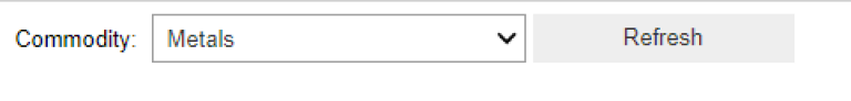
The output looks like the following.
CommodityOverviewWidget(commodities)
References
- developers.lseg.com. 2025. Datastream Web Service | LSEG Developers. [online] Available at: https://developers.lseg.com/en/api-catalog/eikon/datastream-web-service [Accessed 5 March 2025].
- Kumar, A., 2020. Python: How to Add a Trend Line to a Line Chart/Graph - DZone Big Data. [online] dzone.com. Available at: https://dzone.com/articles/python-how-to-add-trend-line-to-line-chartgraph [Accessed 5 March 2021].
- Product.datastream.com. 2020. Datastream Login. [online] Available at: http://product.datastream.com/browse/ [Accessed 12 June 2020].
Get In Touch
Source Code
Related APIs
Request Free Trial
Call your local sales team
Americas
All countries (toll free): +1 800 427 7570
Brazil: +55 11 47009629
Argentina: +54 11 53546700
Chile: +56 2 24838932
Mexico: +52 55 80005740
Colombia: +57 1 4419404
Europe, Middle East, Africa
Europe: +442045302020
Africa: +27 11 775 3188
Middle East & North Africa: 800035704182
Asia Pacific (Sub-Regional)
Australia & Pacific Islands: +612 8066 2494
China mainland: +86 10 6627 1095
Hong Kong & Macau: +852 3077 5499
India, Bangladesh, Nepal, Maldives & Sri Lanka:
+91 22 6180 7525
Indonesia: +622150960350
Japan: +813 6743 6515
Korea: +822 3478 4303
Malaysia & Brunei: +603 7 724 0502
New Zealand: +64 9913 6203
Philippines: 180 089 094 050 (Globe) or
180 014 410 639 (PLDT)
Singapore and all non-listed ASEAN Countries:
+65 6415 5484
Taiwan: +886 2 7734 4677
Thailand & Laos: +662 844 9576