
Author:

Jason Ramchandani
Lead Developer Advocate
Lead Developer Advocate
Last Updated: July 2025
Automating Technical Analysis & Systematic BackTesting of Trading Strategies with Python
In this article I will be using some awesome packages to show you how simple it is to get started with automating the generation of technical analysis features. I will then go on to use these features to generate some simple systematic trading strategies that I will then backtest. This is about the simplest workflow that I have seen for this. I hope you will be pleasantly surprised.
Techincal Analysis
Technical Analysis is the study of investments using prices, volumes and other derived data point histories. As a time-honoured discipline, over the years many indicators have been produced from all parts of the globe. Long the preserve of human eyeballs - the advent of computing in finance has changed the technical analysis landscape with a new level of rigour - leading to the emergence of Systematic Trading and Investment - now well established and the emergent field of AI-first finance - which could leverage such features for Machine Learning. The spread of Python has greatly democratised such pursuits - making them easier than ever to master.
Sections
Implement Candlestick Pattern Recognition
Pre-requisites:
LSEG Workspace with access to LSEG Data Library for Python (Free Trial Available)
Python 3.x
Required Python Packages: LSEG Data Libraries, pandas, numpy, matplotlib, TA-Lib, pandas_ta, mplfinance, backtrader
Import all the packages we need
import lseg.data as ld
import talib
import pandas_ta as pta
import backtrader as bt
import pandas as pd
import matplotlib.pyplot as plt
import matplotlib as mpl
import mplfinance as mpf
import datetime as dt
import numpy as np
import warnings
warnings.simplefilter("ignore")
%matplotlib inline
plt.style.use("dark_background")
mpl.style.use("dark_background")
ld.open_session(app_key="<APP KEY>")
Get our data - one Line API call
Here we use our get_timeseries function to return us hourly OHLCV for cable (GBP=). As FX doesn't carry volume directly - we can use count as a surrogate. We then rename the columns so they can work with charting and backtesting software downstream. Note the dataframe comes back already indexed on timestamp.
RIC = ['GBP=']
start_date = '2025-01-10'
end_date = '2025-06-27'
df1 = ld.get_history(
universe=RIC,
fields = ['OPEN_BID','BID_HIGH_1','BID_LOW_1','BID','BID_NUMMOV'],
start = start_date,
end = end_date,
interval = '1h')
df1.columns=['open','high','low','close','volume']
df1
| open | high | low | close | volume | |
|---|---|---|---|---|---|
| Date | |||||
| 2025-01-10 00:00:00 | 1.2307 | 1.231 | 1.2295 | 1.2295 | 941 |
| 2025-01-10 01:00:00 | 1.2298 | 1.2304 | 1.2291 | 1.2294 | 1696 |
| 2025-01-10 02:00:00 | 1.2295 | 1.2308 | 1.2292 | 1.2301 | 2270 |
| 2025-01-10 03:00:00 | 1.2302 | 1.2307 | 1.2297 | 1.2303 | 1807 |
| 2025-01-10 04:00:00 | 1.2303 | 1.2305 | 1.2297 | 1.2299 | 1483 |
| ... | ... | ... | ... | ... | ... |
| 2025-06-26 20:00:00 | 1.3746 | 1.3748 | 1.3725 | 1.3731 | 3499 |
| 2025-06-26 21:00:00 | 1.3732 | 1.3736 | 1.3719 | 1.3731 | 2160 |
| 2025-06-26 22:00:00 | 1.3727 | 1.3732 | 1.3719 | 1.3726 | 1794 |
| 2025-06-26 23:00:00 | 1.3726 | 1.3728 | 1.3709 | 1.3716 | 1940 |
| 2025-06-27 00:00:00 | 1.3717 | 1.373 | 1.3712 | 1.3721 | 2488 |
2947 rows × 5 columns
df1.dropna(how="any", inplace=True)
len(df1)
2946
Pandas TA package is very useful tool to create various technical analysis features with ease
Types of Indicator
Cycles(1), Momentum(41), Overlap(33), Performance(3), Statistics(11), Trend(18), Utility(5), Volatility(14), Volume(15) as well as Candlestick Patterns (64) are provided by the package ready for you to implement - and as we will see implementation is a breeze. The breadth of indicators means that you can experiment to your hearts content with combinations of indicators etc. We can look at what these are as below:
df1.ta.indicators()
Pandas TA - Technical Analysis Indicators - v0.3.14b0
Total Indicators & Utilities: 205
Abbreviations:
aberration, above, above_value, accbands, ad, adosc, adx, alma, amat, ao, aobv, apo, aroon, atr, bbands, below, below_value, bias, bop, brar, cci, cdl_pattern, cdl_z, cfo, cg, chop, cksp, cmf, cmo, coppock, cross, cross_value, cti, decay, decreasing, dema, dm, donchian, dpo, ebsw, efi, ema, entropy, eom, er, eri, fisher, fwma, ha, hilo, hl2, hlc3, hma, hwc, hwma, ichimoku, increasing, inertia, jma, kama, kc, kdj, kst, kurtosis, kvo, linreg, log_return, long_run, macd, mad, massi, mcgd, median, mfi, midpoint, midprice, mom, natr, nvi, obv, ohlc4, pdist, percent_return, pgo, ppo, psar, psl, pvi, pvo, pvol, pvr, pvt, pwma, qqe, qstick, quantile, rma, roc, rsi, rsx, rvgi, rvi, short_run, sinwma, skew, slope, sma, smi, squeeze, squeeze_pro, ssf, stc, stdev, stoch, stochrsi, supertrend, swma, t3, td_seq, tema, thermo, tos_stdevall, trima, trix, true_range, tsi, tsignals, ttm_trend, ui, uo, variance, vhf, vidya, vortex, vp, vwap, vwma, wcp, willr, wma, xsignals, zlma, zscore
Candle Patterns:
2crows, 3blackcrows, 3inside, 3linestrike, 3outside, 3starsinsouth, 3whitesoldiers, abandonedbaby, advanceblock, belthold, breakaway, closingmarubozu, concealbabyswall, counterattack, darkcloudcover, doji, dojistar, dragonflydoji, engulfing, eveningdojistar, eveningstar, gapsidesidewhite, gravestonedoji, hammer, hangingman, harami, haramicross, highwave, hikkake, hikkakemod, homingpigeon, identical3crows, inneck, inside, invertedhammer, kicking, kickingbylength, ladderbottom, longleggeddoji, longline, marubozu, matchinglow, mathold, morningdojistar, morningstar, onneck, piercing, rickshawman, risefall3methods, separatinglines, shootingstar, shortline, spinningtop, stalledpattern, sticksandwich, takuri, tasukigap, thrusting, tristar, unique3river, upsidegap2crows, xsidegap3methods
Lets see how easy it is to create some Bollinger Bands
Here we will use a popular indicator in the volatility catergory - Bollinger Bands. First we will make a copy of our base price dataframe and then append the bollinger bands feature to the new dataframe. We pass some parameters such as window length of 50 periods, using an simple moving average. We can see the BBL (lower), BBM (mid) and BBU (upper) features, amongst others added to the right of the frame.
df2 = df1.copy()
df2.ta.bbands(length=50, std=2, mamode="sma", ddof=0, append=True)
df2
| open | high | low | close | volume | BBL_50_2.0 | BBM_50_2.0 | BBU_50_2.0 | BBB_50_2.0 | BBP_50_2.0 | |
|---|---|---|---|---|---|---|---|---|---|---|
| Timestamp | ||||||||||
| 2025-01-10 00:00:00 | 1.2298 | 1.2304 | 1.2291 | 1.2294 | 1696 | NaN | NaN | NaN | NaN | <NA> |
| 2025-01-10 01:00:00 | 1.2295 | 1.2308 | 1.2292 | 1.2301 | 2270 | NaN | NaN | NaN | NaN | <NA> |
| 2025-01-10 02:00:00 | 1.2302 | 1.2307 | 1.2297 | 1.2303 | 1807 | NaN | NaN | NaN | NaN | <NA> |
| 2025-01-10 03:00:00 | 1.2303 | 1.2305 | 1.2297 | 1.2299 | 1483 | NaN | NaN | NaN | NaN | <NA> |
| 2025-01-10 04:00:00 | 1.2299 | 1.2303 | 1.2288 | 1.2291 | 1622 | NaN | NaN | NaN | NaN | <NA> |
| ... | ... | ... | ... | ... | ... | ... | ... | ... | ... | ... |
| 2025-06-26 19:00:00 | 1.3746 | 1.3748 | 1.3725 | 1.3731 | 3499 | 1.356026 | 1.366618 | 1.377210 | 1.550155 | 0.805976 |
| 2025-06-26 20:00:00 | 1.3732 | 1.3736 | 1.3719 | 1.3731 | 2160 | 1.356131 | 1.366822 | 1.377513 | 1.564286 | 0.793625 |
| 2025-06-26 21:00:00 | 1.3727 | 1.3732 | 1.3719 | 1.3726 | 1794 | 1.356326 | 1.367038 | 1.377750 | 1.567228 | 0.759608 |
| 2025-06-26 22:00:00 | 1.3726 | 1.3728 | 1.3709 | 1.3716 | 1940 | 1.356591 | 1.367246 | 1.377901 | 1.558537 | 0.704326 |
| 2025-06-26 23:00:00 | 1.3717 | 1.373 | 1.3712 | 1.3721 | 2488 | 1.356888 | 1.367470 | 1.378052 | 1.547693 | 0.718765 |
2946 rows × 10 columns
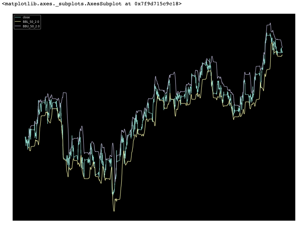
We can now easily plot these as one would in a WorkSpace chart - its not as polished as the WorkSpace chart - but this is for programmatic usage mainly as opposed to in-depth interactive detailed visualisation.
df2[['close','BBL_50_2.0','BBU_50_2.0']].plot(figsize=(18,15))
Candlestick pattern recognition
As we noted earlier there are 64 candlestick patterns that can be identified in both bullish and bearish configurations. Bullish structures are indicated with +100 and bearish structures are indicated with -100. In our case we are using hourly data so we are notified in the hourly row when the signal was generated. Again we simply make a copy of our original prices frame and then append all candlestick patters to that dataframe. One can of course select only the indicators you are interested in.
df3 = df1.copy()
df3.ta.cdl_pattern(name=["2crows", "3blackcrows", "3inside",
"3linestrike", "3outside", "3starsinsouth",
"3whitesoldiers", "abandonedbaby", "advanceblock",
"belthold", "breakaway", "closingmarubozu",
"concealbabyswall", "counterattack", "darkcloudcover"],append=True)
df3
| open | high | low | close | volume | CDL_2CROWS | CDL_3BLACKCROWS | CDL_3INSIDE | CDL_3LINESTRIKE | CDL_3OUTSIDE | CDL_3STARSINSOUTH | CDL_3WHITESOLDIERS | CDL_ABANDONEDBABY | CDL_ADVANCEBLOCK | CDL_BELTHOLD | CDL_BREAKAWAY | CDL_CLOSINGMARUBOZU | CDL_CONCEALBABYSWALL | CDL_COUNTERATTACK | CDL_DARKCLOUDCOVER | |
|---|---|---|---|---|---|---|---|---|---|---|---|---|---|---|---|---|---|---|---|---|
| Timestamp | ||||||||||||||||||||
| 2025-01-10 00:00:00 | 1.2298 | 1.2304 | 1.2291 | 1.2294 | 1696 | 0.0 | 0.0 | 0.0 | 0.0 | 0.0 | 0.0 | 0.0 | 0.0 | 0.0 | 0.0 | 0.0 | 0.0 | 0.0 | 0.0 | 0.0 |
| 2025-01-10 01:00:00 | 1.2295 | 1.2308 | 1.2292 | 1.2301 | 2270 | 0.0 | 0.0 | 0.0 | 0.0 | 0.0 | 0.0 | 0.0 | 0.0 | 0.0 | 0.0 | 0.0 | 0.0 | 0.0 | 0.0 | 0.0 |
| 2025-01-10 02:00:00 | 1.2302 | 1.2307 | 1.2297 | 1.2303 | 1807 | 0.0 | 0.0 | 0.0 | 0.0 | 0.0 | 0.0 | 0.0 | 0.0 | 0.0 | 0.0 | 0.0 | 0.0 | 0.0 | 0.0 | 0.0 |
| 2025-01-10 03:00:00 | 1.2303 | 1.2305 | 1.2297 | 1.2299 | 1483 | 0.0 | 0.0 | 0.0 | 0.0 | 0.0 | 0.0 | 0.0 | 0.0 | 0.0 | 0.0 | 0.0 | 0.0 | 0.0 | 0.0 | 0.0 |
| 2025-01-10 04:00:00 | 1.2299 | 1.2303 | 1.2288 | 1.2291 | 1622 | 0.0 | 0.0 | 0.0 | 0.0 | 0.0 | 0.0 | 0.0 | 0.0 | 0.0 | 0.0 | 0.0 | 0.0 | 0.0 | 0.0 | 0.0 |
| ... | ... | ... | ... | ... | ... | ... | ... | ... | ... | ... | ... | ... | ... | ... | ... | ... | ... | ... | ... | ... |
| 2025-06-26 19:00:00 | 1.3746 | 1.3748 | 1.3725 | 1.3731 | 3499 | 0.0 | 0.0 | 0.0 | 0.0 | 0.0 | 0.0 | 0.0 | 0.0 | 0.0 | -100.0 | 0.0 | 0.0 | 0.0 | 0.0 | 0.0 |
| 2025-06-26 20:00:00 | 1.3732 | 1.3736 | 1.3719 | 1.3731 | 2160 | 0.0 | 0.0 | 0.0 | 0.0 | 0.0 | 0.0 | 0.0 | 0.0 | 0.0 | 0.0 | 0.0 | 0.0 | 0.0 | 0.0 | 0.0 |
| 2025-06-26 21:00:00 | 1.3727 | 1.3732 | 1.3719 | 1.3726 | 1794 | 0.0 | 0.0 | 0.0 | 0.0 | 0.0 | 0.0 | 0.0 | 0.0 | 0.0 | 0.0 | 0.0 | 0.0 | 0.0 | 0.0 | 0.0 |
| 2025-06-26 22:00:00 | 1.3726 | 1.3728 | 1.3709 | 1.3716 | 1940 | 0.0 | 0.0 | 0.0 | 0.0 | 0.0 | 0.0 | 0.0 | 0.0 | 0.0 | -100.0 | 0.0 | 0.0 | 0.0 | 0.0 | 0.0 |
| 2025-06-26 23:00:00 | 1.3717 | 1.373 | 1.3712 | 1.3721 | 2488 | 0.0 | 0.0 | 0.0 | 0.0 | 0.0 | 0.0 | 0.0 | 0.0 | 0.0 | 0.0 | 0.0 | 0.0 | 0.0 | 0.0 | 0.0 |
2946 rows × 20 columns
It can be a bit difficult to see when these signals are being generated from large dataframes - so you can check the min and max readings to see if any bullish or bearish signals are present.
df3.describe()
| open | high | low | close | volume | CDL_2CROWS | CDL_3BLACKCROWS | CDL_3INSIDE | CDL_3LINESTRIKE | CDL_3OUTSIDE | CDL_3STARSINSOUTH | CDL_3WHITESOLDIERS | CDL_ABANDONEDBABY | CDL_ADVANCEBLOCK | CDL_BELTHOLD | CDL_BREAKAWAY | CDL_CLOSINGMARUBOZU | CDL_CONCEALBABYSWALL | CDL_COUNTERATTACK | CDL_DARKCLOUDCOVER | |
|---|---|---|---|---|---|---|---|---|---|---|---|---|---|---|---|---|---|---|---|---|
| count | 2946.0 | 2946.0 | 2946.0 | 2946.0 | 2946.0 | 2946.0 | 2946.0 | 2946.000000 | 2946.000000 | 2946.000000 | 2946.0 | 2946.0 | 2946.0 | 2946.000000 | 2946.000000 | 2946.0 | 2946.000000 | 2946.0 | 2946.0 | 2946.000000 |
| mean | 1.299157 | 1.30027 | 1.298116 | 1.2992 | 3890.517651 | 0.0 | 0.0 | 0.135777 | 0.101833 | -0.882553 | 0.0 | 0.0 | 0.0 | -1.120163 | 0.135777 | 0.0 | 0.305499 | 0.0 | 0.0 | -0.033944 |
| std | 0.043508 | 0.043482 | 0.043526 | 0.043514 | 1913.721285 | 0.0 | 0.0 | 8.642016 | 3.190044 | 17.459197 | 0.0 | 0.0 | 0.0 | 10.526117 | 29.018732 | 0.0 | 25.061724 | 0.0 | 0.0 | 1.842399 |
| min | 1.2105 | 1.2132 | 1.2097 | 1.2106 | 1.0 | 0.0 | 0.0 | -100.000000 | 0.000000 | -100.000000 | 0.0 | 0.0 | 0.0 | -100.000000 | -100.000000 | 0.0 | -100.000000 | 0.0 | 0.0 | -100.000000 |
| 25% | 1.2607 | 1.2615 | 1.2598 | 1.2607 | 2507.0 | 0.0 | 0.0 | 0.000000 | 0.000000 | 0.000000 | 0.0 | 0.0 | 0.0 | 0.000000 | 0.000000 | 0.0 | 0.000000 | 0.0 | 0.0 | 0.000000 |
| 50% | 1.2965 | 1.2974 | 1.2957 | 1.2965 | 3883.0 | 0.0 | 0.0 | 0.000000 | 0.000000 | 0.000000 | 0.0 | 0.0 | 0.0 | 0.000000 | 0.000000 | 0.0 | 0.000000 | 0.0 | 0.0 | 0.000000 |
| 75% | 1.3377 | 1.338675 | 1.3367 | 1.337775 | 5125.0 | 0.0 | 0.0 | 0.000000 | 0.000000 | 0.000000 | 0.0 | 0.0 | 0.0 | 0.000000 | 0.000000 | 0.0 | 0.000000 | 0.0 | 0.0 | 0.000000 |
| max | 1.3756 | 1.377 | 1.375 | 1.3756 | 12774.0 | 0.0 | 0.0 | 100.000000 | 100.000000 | 100.000000 | 0.0 | 0.0 | 0.0 | 0.000000 | 100.000000 | 0.0 | 100.000000 | 0.0 | 0.0 | 0.000000 |
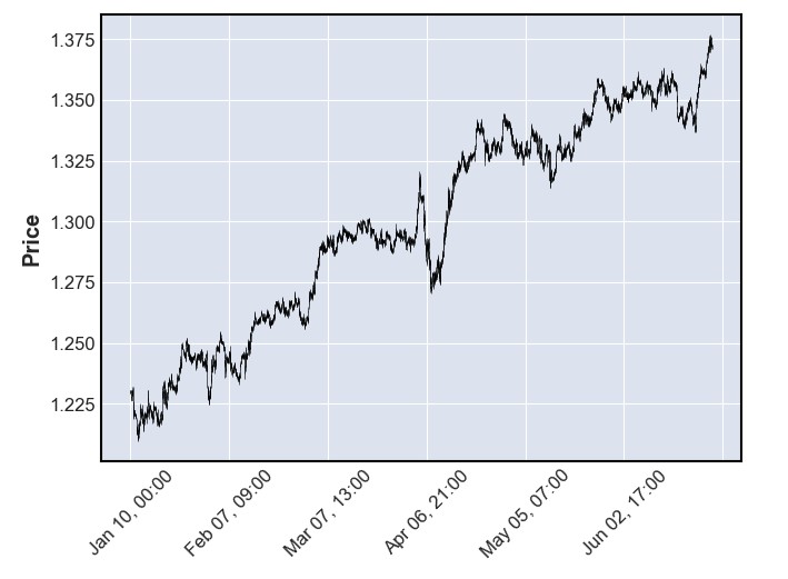
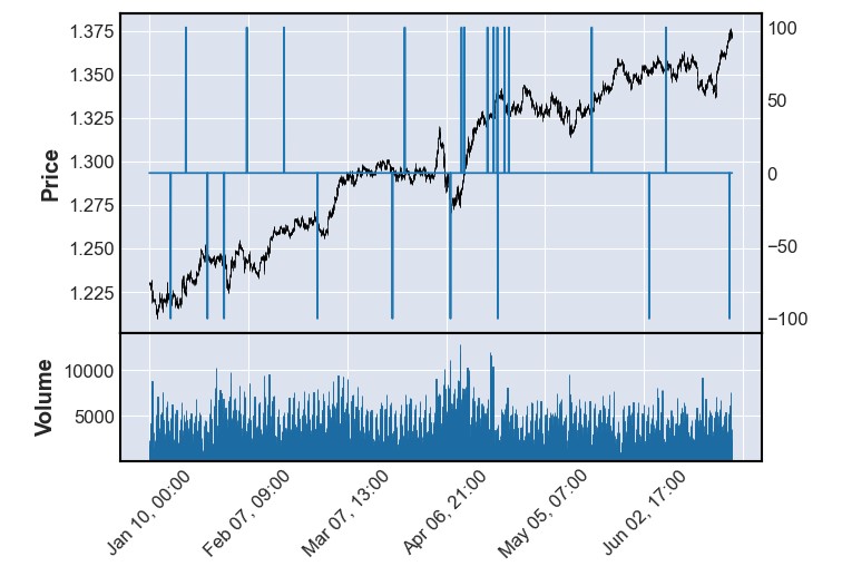
Lets use Matplotlib Finance package to create some candlestick charts with ease
We can use the candlestick charts to help us visualise when these candlestick patterns fire - first lets create a candlestick chart and then overlay a candlestick signal - in our case the CDL_3INSIDE (3 inside candles pattern - which is a compression signal which can present in both bullish (+100) and bearish (-100) variants.
df3 = df3.astype(float)
mpf.plot(df3, type='candle')
apdict = mpf.make_addplot(df3['CDL_3INSIDE'])
mpf.plot(df3,volume=True,addplot=apdict)
Implement backtesting of a strategy using BackTrader package
So we have seen how we can automate the creation of Techincal Analysis indicators very easily from a dataframe of prices. The ease with which we executed this is kind of remarkable. The next stage we can go to - is to use these indicators to create a trading strategy and to then test its efficacy through backtesting. This is also relatively easy to accomplish using the BackTrader package. First lets make a copy of our original dataframe.
df4 = df1.copy()
Set up a simple SMA crossover strategy using built-in strategy
The BackTrader package uses a base strategy class which you can use to inherit from to build your own custom strategy. In our case we will be implementing 2 trading strategies firstly a simple moving average crossover (MA XOver) strategy and then a slightly more complex combinatorial strategy where we only take signals in the direction of the trend.
smaCross strategy
First you can see this is composed of a list of parameter (in our case the window length for the moving averages). Next an init section which defines both the indicators from the bt.ind collection and also the crossover event itself. Note that the cross over event is bidirectional - though one can change this etc. Finally we have the trading logic section which uses the previously defined event signal (crossover signal) and combines it with our position information to inform an action. In our case we have defined to actions -
* If we do not have a position and we have a bullish cross (ie fast sma crosses slow sma from below) then take a position
* If we do have a position and we have a bearish cross (ie fast sma crosses slow sma from above) then close the position
Note - we don't allow shorting in this first strategy for simplicities sake. We will include shorting in the second of our strategies.
class smaCross(bt.Strategy):
# list of parameters which are configurable for the strategy
params = dict(
pfast=50, # period for the fast moving average
pslow=200 # period for the slow moving average
)
def __init__(self):
sma1 = bt.ind.SMA(period=self.p.pfast) # fast moving average
sma2 = bt.ind.SMA(period=self.p.pslow) # slow moving average
self.crossover = bt.ind.CrossOver(sma1, sma2) # crossover signal
def next(self):
if not self.position and self.crossover > 0: # not in the market
self.buy(size=100)
elif self.position and self.crossover < 0: # in the market & cross to the downside
self.close() # close long position
Candle Mix Stategy
Here we extend our basic smaCross strategy by say introducing a candlestick pattern - in this case the 3Inside candlestick pattern.
class cdlmix(bt.Strategy):
# list of parameters which are configurable for the strategy
params = dict(
pfast=50, # period for the fast moving average
pslow=100 # period for the slow moving average
)
def __init__(self):
self.cdl3 = bt.talib.CDL3INSIDE(self.data.open,self.data.high,self.data.low, self.data.close)
self.sma1 = bt.ind.SMA(period=self.p.pfast) # fast moving average
self.sma2 = bt.ind.SMA(period=self.p.pslow) # slow moving average
self.crossover = bt.ind.CrossOver(self.sma1, self.sma2) # crossover signal
def next(self):
if not self.position:
if self.sma1 > self.sma2 and self.cdl3 == 100: # not in the market
self.buy(size=100)
if self.sma1<self.sma2 and self.cdl3 == -100:
self.sell(size=100)
elif self.position.size > 0 and (self.crossover <0 or self.cdl3 == -100): # in the market & cross to the downside
self.close() # close long position
#self.sell(size=100) # Open short
elif self.position.size < 0 and (self.crossover >0 or self.cdl3 == 100): # in the market & cross to the downside
self.close() # close short position
self.buy(size=100) # Open long
Now that we have our two strategies defined - we can pass it to our broker object which we configure to run the strategy we just created. From below we can see that the first section is where we initialise the bt.Cerebro object - setting our initial cash level and also commission rates. Next we add the strategy we just created and then define a data object which we wire up to our pandas dataframe, and specify the from and to dates as datetime objects and as we are using hourly bars we set the timeframe to be minutes with a compression rate of 60. We then add the data to the broker object and run the backtest and finally we format the standard chart output generated.
For easy multiple strategy tests - I have created a generalised brokerObject function from the basic package documentation which takes a number of parameters in order to create a valid backtest of a valid strategy and just configured it to return the cerebro.plot object which contains all the results.
# create a function for this which takes a strategy_name, df, date_from, date_to & time_frame & compression as an input
def brokerObject(strategy_name,data_frame,from_date,to_date,time_frame,compression):
# initialize backtrader broker
cerebro = bt.Cerebro(stdstats=True)
cerebro.broker.setcash(1000)
cerebro.broker.setcommission(commission=0.001)
# add strategy
cerebro.addstrategy(strategy_name)
# wire up bt.feeds.PandasData to data_frame, set timeperiod, timeframe and also compression
data = bt.feeds.PandasData(dataname=data_frame,fromdate=from_date,todate=to_date,
timeframe=time_frame,compression=compression)
cerebro.adddata(data)
# run backtest
res = cerebro.run()
strat = res[0]
#prepare plots
mpl.rcParams['font.sans-serif']=['DejaVu Sans']
mpl.rcParams['axes.unicode_minus']=False
mpl.rcParams['figure.figsize']=[18, 16]
mpl.rcParams['figure.dpi']=200
mpl.rcParams['figure.facecolor']='w'
mpl.rcParams['figure.edgecolor']='k'
return cerebro.plot(style='candle',iplot=False,width=30,height=30,start=from_date, end=to_date)
brokerObject(smaCross,df4,dt.datetime.strptime(start_date, '%Y-%m-%d'),dt.datetime.strptime(end_date, '%Y-%m-%d'),bt.TimeFrame.Minutes,60)
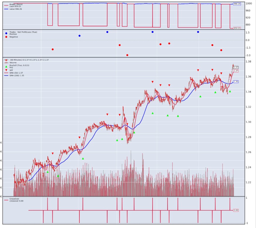
brokerObject(cdlmix,df4,dt.datetime.strptime(start_date, '%Y-%m-%d'),dt.datetime.strptime(end_date, '%Y-%m-%d'),bt.TimeFrame.Minutes,60)
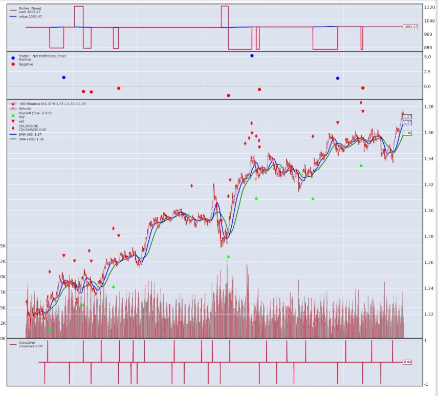
In this article we have seen how we can very easily generate Technical Analysis features using Pandas_TA / TA_Lib packages. These work seamlessly with the output from our LSEG Data Library and are simply appended to the right of the dataframe. We have also seen how we can eyeball these indicators using basic charting in Python. In particular we have shown how we can plot candlestick patterns firing on a chart with real simplicity.
We then went on to take things a little further by creating some simple trading strategies using our indicators in the strategy template of the backtrader package and then wired that up to the backtrader broker object that conducted the backtest for us and outputted a series of plots that visualised the strategy and sig-gen, P&L and such.
This is really the simplest workflow I have seen for backtesting trading strategies - and whilst there are undoubtably more sophisticated packages and approaches - particularly for live streaming strategies - I think this is a great introductory approach and worthy of your attention.
Further Resources
For Content Navigation in Workspace - please use the Data Item Browser Application: Type 'DIB' into Search Bar.
For Python/ AI/ML / Quant Finance / Algo Trading training
Books:
For Technical Analysis training & consultancy - Trevor Neil
Meetup Group
Get In Touch
Source Code
Related Articles
-
Create Technical Analysis triggers and signals using the LSEG Data Library for Python
-
Technical Analysis Indicators: Customisable Relative Strength Indices
-
Generate Charts for Trading Analysis using RDP Historical Pricing Data
-
Simplifying Intraday Market Analysis: Unveiling Insights for Traders and Analysts
Related APIs
Request Free Trial
Call your local sales team
Americas
All countries (toll free): +1 800 427 7570
Brazil: +55 11 47009629
Argentina: +54 11 53546700
Chile: +56 2 24838932
Mexico: +52 55 80005740
Colombia: +57 1 4419404
Europe, Middle East, Africa
Europe: +442045302020
Africa: +27 11 775 3188
Middle East & North Africa: 800035704182
Asia Pacific (Sub-Regional)
Australia & Pacific Islands: +612 8066 2494
China mainland: +86 10 6627 1095
Hong Kong & Macau: +852 3077 5499
India, Bangladesh, Nepal, Maldives & Sri Lanka:
+91 22 6180 7525
Indonesia: +622150960350
Japan: +813 6743 6515
Korea: +822 3478 4303
Malaysia & Brunei: +603 7 724 0502
New Zealand: +64 9913 6203
Philippines: 180 089 094 050 (Globe) or
180 014 410 639 (PLDT)
Singapore and all non-listed ASEAN Countries:
+65 6415 5484
Taiwan: +886 2 7734 4677
Thailand & Laos: +662 844 9576