


Climate change has emerged as the biggest environmental challenge of our time, posing significant risks and opportunities for the financial industry. Investors who are aligning with the objectives of the Paris Agreement, are implementing net zero investment strategies or enhancing their financial risk management processes due to the transition to a low-carbon economy. These investors need to measure, manage and report the emissions of their investment portfolios - referred to as financed emissions.
LSEG Climate data provides granular company reported climate data which is aligned with the latest disclosure and regulatory standards, sophisticated analytics and innovative estimated emissions models covering approximately 90% of the global market capitalization. The hierarchical, multi-model approach to estimating emissions improves the data accuracy, reduces risk of underestimating emissions, and solves the data availability challenge. The transparency of sources and methodologies supports PCAF quality score assessment at a company level. The Partnership for Carbon Accounting Financials (PCAF) is a financial sector initiative, establishing an international standard for calculating the Greenhouse Gas (GHG) Emissions from loans and investments.
The Estimated Emissions methodology used at LSEG is available here.
What data is needed
A company's carbon footprint is a key metric for quantifying its contribution to rising temperatures, as well as its vulnerability in case of a rapid de-carbonization trajectory. There are three complementary categories of emissions:
- Scope 1: These are direct emissions from the sources which are owned or controlled by the reporting company.
- Scope 2: These are indirect emissions due to the consumption of electricity, heat, steam and cooling.
- Scope 3: The indirect emissions from the upstream and downstream activities in the company's value chain or its products life cycle
- Upstream: The emissions from processes in the value chain that contribute to a company's products or services (e.g. purchase of goods and services, upstream freight, employee commute, etc.)
- Downstream: The emissions from the activities of customers using a company's products and services, which includes financed emissions.
Depending on your overall objective, there are several ways to assess financed emissions, each of them serving its own purpose:
- Financed emissions (in tonne CO2eq) represents the total GHG emissions owned by a portfolio through its investee firms. It can be used as an impact metric, to understand the overall climate impact of investments, and set an absolute baseline for GHG mitigation actions.
- Financed emissions intensity (in tonne CO2eq/$M invested) is the financed emissions as described above, divided by the investment volume. It can be useful to compare different investment policies, portfolios, or to track the year on year progress.
- Weighted Average Carbon Intensity (WACI, in tonne CO2eq/$M revenues) is the average of carbon intensity (by revenues) of investee firms, weighted by the portfolio exposure. WACI is used to compare different portfolios and it helps understand exposure to emissions-intensive companies and has been endorsed by TCFD.
One of the primary objectives of GHG emissions accounting is to create transparency for stakeholders. Therefore, being able to assess the quality of the data used to perform carbon foot-printing, and how it translates into the overall quality of the assessed financed emissions, is a critical step on the de-carbonization journey.
In this article, we are using PCAF (2022). The Global GHG Accounting and Reporting Standard Part A: Financed Emissions. Second Edition principles.
Data availability
LSEG provides the Climate data through the bulk file downloads. These bulk files are available through the Client File Services (CFS) API within Data Platform (RDP) and allow a user to get a latest complete snapshot of all the data, as well as any weekly changes from the previous snapshot. The bulk files are delivered in the CSV and JSON format, which allows them to be used with Excel, as well as within an application. This bulk data enables a quick analysis of a portfolio's GHG emissions.
Following Climate data packages are available within CFS bulk (for Quant and IB Full license):
| Package | Description |
| Measures-CDP-Limited-v1 | Contains all CDP data items with values and collection timestamps including links to Source and As reported data for organisations determined to be private when data was collected. |
| Measures-CDP-v1 | Contains all CDP data items with values and collection timestamps including links to Source and As reported data for organisations determined to be public when data was collected. |
| Measures-Full-Limited-v1-DataItems | Contains all Climate data items with values and collection timestamps including links to Source and As reported data for organisations determined to be private when data was collected. |
| Measures-Full-v1-Analytics | All Climate indicators with values and calculation timestamps for organisations determined to be public when data was collected. |
| Measures-Full-v1-DataItems | Contains all Climate data items with values and collection timestamps including links to Source and As reported data for organisations determined to be public when data was collected. |
| Sources-Full-v1 | Descriptive data on the sources of each datapoint value. |
| AsReported-Full-v1 | Descriptive data on the as reported elements of each datapoint value. |
The bulk files are available in two formats:
- JSONL: json line format, with the file extension .jsonl
- CSV: comma separated values format with the file extension .csv
There are two updates types to these files:
- INIT: Full initialization file of all organizations
- DELTA: Refresh of organizations with changed data
All the files are compressed and delivered as a .gz file.
The bulk file used in this article is the Bulk-Climate-Global-Measures-Full-v1-DataItems.
Note: if you have subscription to ESG data with the Climate add-on package, then you should use: Bulk-Climate-Global-Measures-AddOn-v1-DataItems The revenue and EVIC data should be pulled from the ESG bulk data files.
Greenhouse Gas analysis
This article accompanies sample code, which is provided as a Python notebook. The notebook downloads and uses the CFS bulk data files described above. The input to the notebook is a portfolio of user's choice and it performs following analysis for a well rounded picture of the GHG exposure:
- Percentage of portfolio which has climate data coverage
- Weighted Average Carbon Intensity (WACI)
- Financed Emissions
- PCAF Data quality score
The first task in the sample is to download the Climate bulk file and extract the fields of interest. This is a one time process and so the code is listed at the end of the notebook. The data fields of interest and the corresponding value containers are mapped. The code downloads all the files in this package and iterates over the JSON entries eventually building a Pandas dataframe. Finally this dataframe is stored as a pickle file and can be used multiple times for portfolio analysis.
# parse out the entries in the bulk file
climateData = []
for cMeasuresFile in bFiles:
for l in cMeasuresFile.splitlines():
jObj = json.loads(l)
# build a dictionary of field/value pairs
for measure in jObj['ESGMeasureValue']['EsgMeasureValues']:
dt[measure['EsgDataMeasure']] = measure['EsgDatapointValue'][fields[measure['EsgDataMeasure']]]
dt['OrganizationId'] = jObj['ESGStatementDetails']['OrganizationId']
dt['FinancialPeriodFiscalYear'] = jObj['ESGStatementDetails']['FinancialPeriodFiscalYear']
climateData.append(dt)
The primary identifier of a company in this data is PermID, shown as the field OrganizationId. If the portfolio contains RIC or ISIN etc, the Symbology API should be used to lookup the corresponding PermID of the holdings. Complete example of how to do so is shown in the sample code.
Load the target portfolio
The portfolio data is expected in a CSV file format and contains two columns - RIC and Weight. The weights should sum up to 100%. Once we have the portfolio, we can use the RDP symbology convert service to get the Organization PermID and the Reporting Currency, and add this data into the portfolio dataframe. The symbology service REST endpoint is /data/symbology/beta1/convert. This service limits the number of instruments that can be converted in a single call - hence a bigger list of instruments is divided into chunks of 90 each.
portfolio = pd.read_csv('Portfolio.csv')
RIClist = portfolio['RIC'].tolist()
bucketSize = 90
buckets = [ RIClist[i: i + bucketSize] for i in range(0, len(RIClist), bucketSize) ]
for bucket in buckets:
reqData = {
"universe": bucket,
"to": ["OrganizationId"]
}
hResp = postRequest('/data/symbology/beta1/convert', reqData)
The portfolio used in the following illustrations is the FTSE All World Index, with a 1 million USD investment.
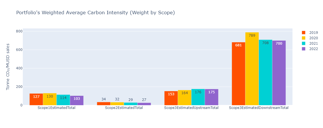
Weighted Average Carbon Intensity (WACI)
As stated above, WACI is defined as the average of carbon intensity (by revenues) of portfolio holdings, weighted by the portfolio exposure. Therefore, theoretical WACI = $ \sum_{Portfolio}Weight \text{ } * \text{ } {GHG \text{ } Emissions \over Revenue} $
In practice, it is important to rebase the WACI, since the GHG emissions data might not be available for 100% of a portfolio. Rebaselining will allow for better comparisons like year on year changes or comparing with a benchmark. The modified formula for rebased WACI is to divide the above result with the actual GHG emissions data coverage.
WACI = ${\sum_{Portfolio}Weight \text{ } * \text{ } {GHG \text{ } Emissions \over Revenue} \over \sum_{Portfolio}Weight \text{ } (GHG \text{ } Emissions \text{ } or \text{ } Revenue \neq 0)} $
This above formula is realized in the code as follows:
# tPort is the climate data for a specific year merged into the portfolio dataframe
# get a subset of dataframe where climate and revenue data are both available
sDF = tPort[tPort[measure].notna() & tPort['SalesinUSD'].notna() & (tPort['SalesinUSD'] != 0)]
# measure is one of the scopes for which WACI is to be calculated
neu = (sDF['Weight'] * sDF[measure] / (sDF['SalesinUSD'] / 1000000)).sum()
deno = sDF['Weight'].sum()
waci = neu/deno
Based on the following coverage:
| Coverage | 2019 | 2020 | 2021 | 2022 |
| Scope 1 | 97.71% | 98.37% | 98.45% | 82.46% |
| Scope 2 | 97.71% | 98.37% | 98.45% | 82.46% |
| Scope 3 Upstream | 84.14% | 84.79% | 85.00% | 69.89% |
| Scope 3 Downstream | 84.14% | 84.79% | 85.00% | 69.89% |
Note: Since the data is always changing and new instruments are being added, your results might be different.
As is evident in this bar chart, there is a gap in coverage between Scope 1, 2 and Scope 3. This is mainly due to the fact that our model does not currently provide estimates for the Financial industry. An alternative method would be to consider the values, only when we have an estimate across all GHG emissions scope.
Financed emissions
To assess the Financed emissions, we're using PCAF methodology:
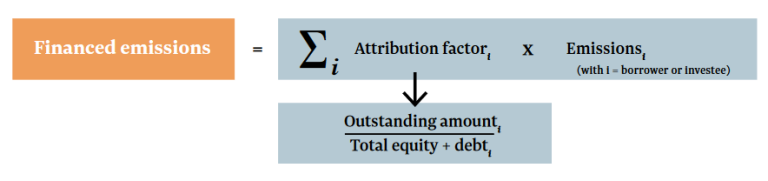
where the attribution factor is $ Outstanding \text{ } Amount \over EVIC $, EVIC being Enterprise Value Including Cash. As with the WACI example, we are considering an investment of 1M USD in FTSE All World Index.
Theoretical Financed Emissions = $ \sum_{Portfolio} GHG \text{ } Emissions \text{ } * \text{ } {Constituent \text{ } Weight \text{ } * \text{ } Amount \text{ } Invested \over EVIC} $. Again, we need to rebaseline our result due to the GHG emissions coverage being less than 100%.
This above formula is realized in the code as follows:
# tPort is the climate data for a specific year merged into the portfolio dataframe
# get a subset of dataframe where climate and EVIC are both available
sDF = tPort[tPort[measure].notna() & tPort['EnterpriseValueincludingCashandShortTermInvestmentsinUSD'].notna() & (tPort['EnterpriseValueincludingCashandShortTermInvestmentsinUSD'] != 0)]
# measure is one of the scopes for which FE is to be calculated
neu = (sDF[measure] * PortfolioAmountInvested * sDF['Weight'] / sDF['EnterpriseValueincludingCashandShortTermInvestmentsinUSD'] ).sum()
deno = sDF['Weight'].sum()
fe = neu/deno
Doing that independently for Scope 1, Scope 2, Scope 3 Upstream and Downstream, we get:
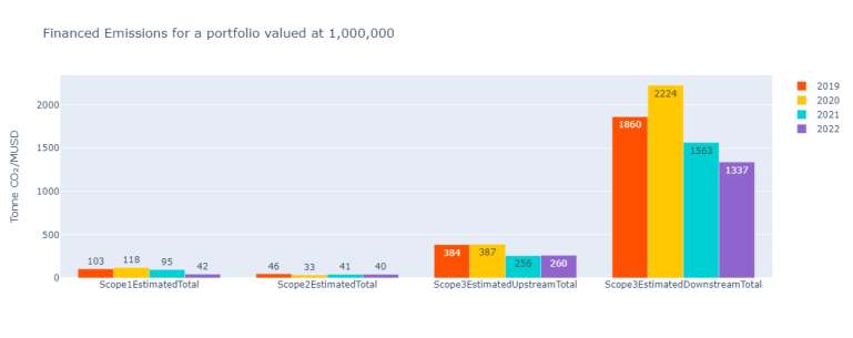
The coverage is slightly different from WACI calculations, due to a lack of EVIC for some corporations.
| Coverage | 2019 | 2020 | 2021 | 2022 |
| Scope 1 | 97.33% | 98.23% | 98.20% | 57.79% |
| Scope 2 | 97.33% | 98.23% | 98.20% | 57.79% |
| Scope 3 Upstream | 83.79% | 84.68% | 84.75% | 50.38% |
| Scope 3 Downstream | 83.79% | 84.68% | 84.75% | 50.38% |
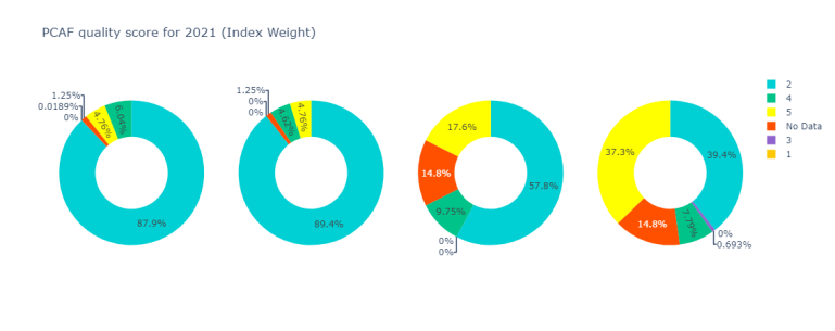
PCAF Data quality score
Finally, following the PCAF recommendations, it's important to provide the stakeholders with information regarding the data quality of the GHG emissions used to calculate the Financed emissions. PCAF provides the following table, Score 1 being the highest quality data and Score 5 the lowest:
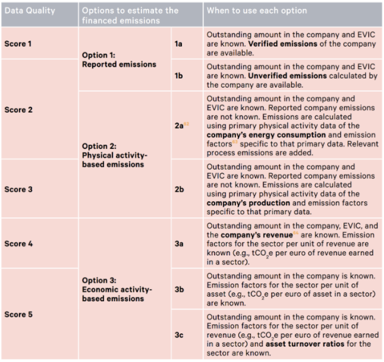
As described in the methodology document, a hierarchical multi-model approach regarding GHG emissions estimations has been adopted. The source of the data is being disclosed along with the value itself. Based on this, we have the following correspondence with PCAF Data Quality scores:
| Scope | Field value | Score |
| All | Reported_value | 2 |
| All | Winsorized | 4 |
| All | Extrapolated | 4 |
| All | Aggregated_model | 5 |
| Scope 1 | Energy_model | 3 |
| Scope 1 | Energy_extrapolated | 4 |
| Scope 3 Downstream | Fossil_fuel_production_model | 3 |
We then now assess financed emissions against these scores. This is achieved in the following code snippet.
scoresByWeight = [0] * numberScoreGrades
# aggregate all the weights for a particular score
sDF = tPort[tPort['EnterpriseValueincludingCashandShortTermInvestmentsinUSD'].notna() & (tPort['EnterpriseValueincludingCashandShortTermInvestmentsinUSD'] != 0)]
for grade in range(numberScoreGrades):
scoresByWeight[grade] = sDF[sDF[scope] == grade]['Weight'].sum()
# add the weights which don't have enterprise value into the n/a bucket
sDF = tPort[tPort['EnterpriseValueincludingCashandShortTermInvestmentsinUSD'].isna() | (tPort['EnterpriseValueincludingCashandShortTermInvestmentsinUSD'] == 0)]
scoresByWeight[0] += sDF['Weight'].sum()
return scoresByWeight
Here for year 2021, we are also taking into account the rebaselined financed emissions for which no data was available.
and
Summary
LSEG climate data can be used to calculate standard or custom scores and grades. The complete sample Python notebook used in this article can be downloaded from LSEG API Sample GitHub Repo.