
Quantum computing is expected to impact many industries including financial services and cyber-security [1]. Drawing from quantum mechanics concepts, relating to phenomena such as superposition, entanglement and interference, quantum computing is expected to be able to tackle problems at a scale and granularity that classical computing may have difficulty exploring.
Leveraging on its prior experiences in classical computing, the research community is evolving the ecosystem very fast, showcasing significant progress such as Microsoft's recent milestone announced on the development of the Majorana 1 chip [2]. Such progress, demonstrates that we are now moving towards the emergence of the next generation of quantum, from NISQ hardware to resilient quantum structures, and closer to Quantum at scale.
Quantum financial services
Early on, the financial industry has started exploring the benefits of Quantum computing and many prototypes have been introduced exploring the quantum advantage in context. Business projections, place the industry value at around 200 billion USD by 2040 [3].
Existing use cases in financial services include derivatives pricing, financial market indicators, optimisations, settlements and Quantum AI.
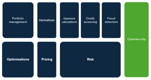
We identify four main pillars where Quantum computing can be utilised within the financial services industry:
- Optimisations
- Pricing and valuations
- Risk
- Cybersecurity
There are many use cases amongst all pillars that can potentialy benefit from the Quantum advantage, from asset allocations and optimisations, options or warrants valuations, to risk exposure stress tests and simulations. Amongst all applications, we can find some common methodologies in their algorithmic solutions. For example, Quadratic programming and Monte Carlo methods are often utilised at some step of such use cases.
Variational Quantum Eigensolvers
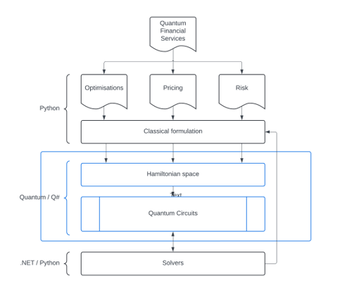
In this article, we propose a process that can bridge classical problems with quantum computing to streamline the delivery of quantum circuits executing such algorithms within financial use cases. We use python, as an established language within financial services, to drive the use cases to the point where a quantum circuit is injected in the pipeline. Mathematical transformations convert the problem from its classical layer to a quantum representation space. Thereafter, we use Microsoft Q# to transparently generate the appropriate quantum circuits and run the desired algorithms within the Quantum space. The generated Ansatz provides an initial calculation of the expected value, and the results are passed back to the classical layers into classical optimisers that close the loop that drives the structures of the quantum circuits. Such hybrid structures are called Variational Quantum Eigensolvers (VQEs).
We begin our journey by trying to solve a simple use case within the financial optimisations ecosystem, that of the binary portfolio selection. In more detail, for the purposes of this article, we will be:
- Expressing the classical problem using a cost function form, by utilizing PyQUBO which will derive the appropriate Classical to Quantum translation matrix Q.
- Using Q to express the cost Hamiltonian in exponential form.
- Writing a Q# dynamic algorithm able to:
a. Generate quantum register rotations.
b. Generate the Mixer Hamiltonian.
c. Connect a Hadamard layer with Hc and Hm and re-iterate if appropriate.
d. Execute the ansatz and collect the results.
What you will need
Let’s start by importing the appropriate libraries:
import lseg.data as ld
import pandas as pd
import numpy as np
import matplotlib.pyplot as plt
import qsharp
from pyqubo import Array, Placeholder, Constraint
from Quantum.quantum_helpers import qubo_to_ising, qubo_to_str_array
Ingesting the data
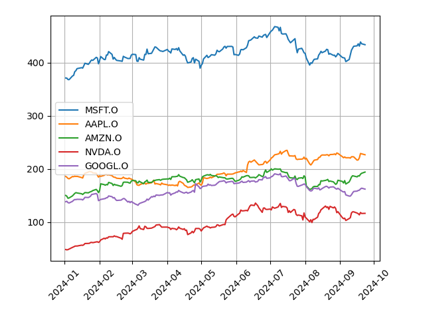
We will be ingesting historical prices for five different instruments. We will be using 2024 Nasdaq closing prices for Microsoft, Nvidia, Apple, Amazon and Google. To ingest the data, we use the LSEG data libraries for python:
rics = [
'MSFT.O',
'AAPL.O',
'AMZN.O',
'NVDA.O',
'GOOGL.O'
]
try:
df = pickle.load(open('./data/lseg_intraday_data.pkl', 'rb'))
except:
ld.open_session()
df = ld.get_history(universe=rics, # RICS universe
fields="TRDPRC_1",
start='2024-01-01’, # start date
end='2024-09-23', # end date
interval="1d") # bar length
ld.close_session()
pickle.dump(data, open(f'./data/lseg_intraday_data.pkl', 'wb'))
Let’s now plot the stock prices for the five instruments:
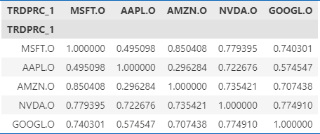
We then calculate the correlations matrix for these instruments historical price movements which will later use in the classical formulation of our QUBO model:
correlation_matrix = df.corr()
corr = correlation_matrix.to_numpy()
correlation_matrix
The QUBO and Ising model
New types of computational technologies such as Quantum computers require new formulations of classical problems. In the classical space the binary portfolio optimisation can be solved using any module supporting Quadratic Unconstrained Binary Optimisation (QUBO) calculations. In the Quantum space, we need to prepare the equivalent of a classical cost function, an energy function called the Hamiltonian. To transition between the two worlds, we will be using the pyQUBO library allowing us to formulate a mathematical QUBO problem and its Hamiltonian - the ising model. The following code snippet, implements this process:
assets = df.columns
mu = df.mean()
n_assets = len(assets)
x = Array.create('x', shape=n_assets, vartype= 'BINARY')
HProfit = 0.0
for i in range(n_assets):
HProfit += Constraint(mu[rics[i]]*x[i], label='Profit({})'.format(i))
HRisk = 0.0
for i in range(n_assets):
for j in range(i+1, n_assets):
HRisk += Constraint(corr[i][j]*x[i]*x[j], label='Risk({},{})'.format(i, j))
theta = Placeholder('theta')
HModel = H.compile()
On the above snippet, we can see several phases formulating the classical QUBO problem. First the profit for each asset is expressed in the HProfit constraint. We then inject the HRisk constraint simulating the risk carried through the covariance matrix and formulate our Hamiltonian function using theta as a risk diversification parameter:
H = Hprofit + theta * Hrisk
We can then obtain the QUBO form by running the to_qubo function:
theta = 0.5
model_dict = {'theta':theta}
Q, offset = HModel.to_qubo(feed_dict = model_dict, index_label=True)
print(f"Proprietary pyQUBO Q\n{Q}")
One of the outputs of the PyQUBO process is the Q matrix, this is our connection point to Quantum. What we now need is to convert this problem into its ising format. We can then pass Pauli matrices and weights into Q# and the appropriate algorithm that will drive the quantum circuit generation.
Q, strQ = qubo_to_str_array(Q, n_assets)
print(f"Reconstructed Q:\n {Q}")
pauli, weights, offset = qubo_to_ising(Q)
print(f"Pauli matrices:\n{pauli}")
print(f"Weights:\n{weights}")
Quantum Approximate Optimisation Algorithm
The Quantum Approximate Optimisation Algorithm (QAOA) algorithm is a variational quantum algorithm that can be used in combinatorial optimisation problems. QAOA encodes the Hamiltonian function into the appropriate Quantum circuit. A single QAOA layer consists of two consecutive layers called the Hamiltonian layer and a mixer layer. The following Q# function is able to dynamically build the appropriate Quantum circuit given the ising equivalent of a QUBO formulation. It can also be used to build stacked structures of the layer to generate deeper circuits:
operation QAOA(b:Double[], pauli:Double[][], w:Double[], n_layers:Int) : Result[] {
let n_qubits = Length(pauli[0]);
use quantum_register = Qubit[n_qubits];
// Apply Hadamard layer once
for i in 0..n_qubits - 1 {
H(quantum_register[i]);
}
// Apply Hc-Hm n_layers deep
for l in 0..n_layers - 1 {
// Apply Hamiltonian cost
for j in 0..Length(pauli) - 1 {
let current_pauli_term = pauli[j];
mutable ix_ones = [0, size= n_qubits];
mutable ix = 0;
for k in 0..Length(current_pauli_term) - 1 {
if current_pauli_term[k] == 1.0 {
set ix_ones = ( ix_ones w/ ix <- k) ;
set ix += 1;
}
}
if ix == 1 {
R(PauliZ, 2.0 * b[l] * w[j], quantum_register[j]);
}
elif ix == 2 {
Rzz(2.0 * b[l] * w[j], quantum_register[ix_ones[0]], quantum_register[ix_ones[1]]);
}
}
// Apply Hamiltonian mixer
for i in 0..n_qubits - 1 {
R(PauliX, 2.0 * b[l], quantum_register[i]);
}
}
DumpRegister(quantum_register);
let result = MResetEachZ(quantum_register);
return result;
}
We next initiate the integration with Q# and execute the QAOA function that generates the circuit and passes that to the Microsoft quantum simulator:
qsharp.init(project_root='./Quantum/')
layer_parameters = "[0.25, 0.35]"
eval_fn = f"QAOA.QAOA({layer_parameters}, {pauli} , {weights}, 2)"
print(eval_fn)
print(qsharp.eval(eval_fn));
The execution of the function renders the following results:
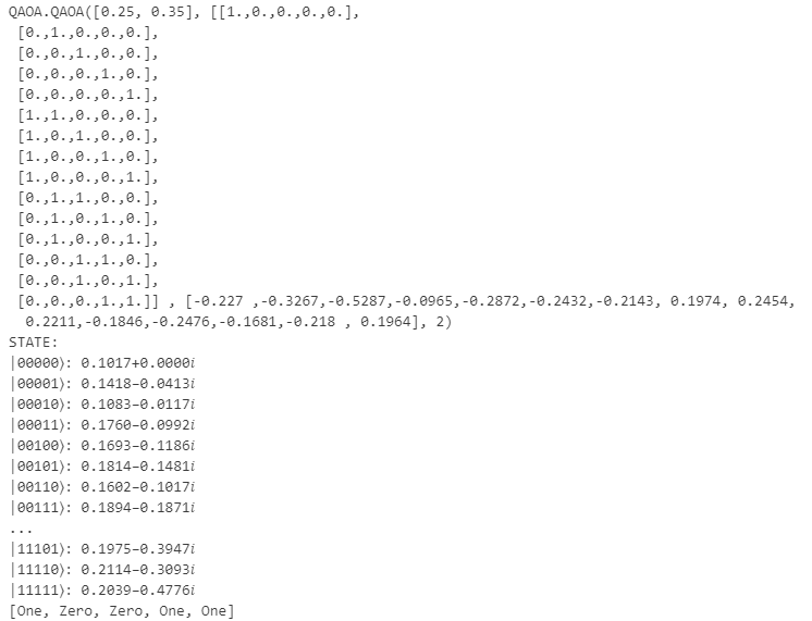
We can see the solution vector resulting from the quantum simulation is [1, 0, 0, 1, 1]. Those, given the small financial dataset provided, would be stocks MSFT.O, NVDA.O and GOOGL.O, we should also mention that this algorithm explores only the binary participation of stocks within a portfolio.
Future work
Future work could include closing the loop from quantum to classical by adding an optimisation layer of the quantum results, a new Q# function able to build a Monte Carlo Quantum circuit that can be used to perform a full Quantum portfolio optimisation with continuous weighting. Such an attempt could potentially surface how we could better explore the data space, resulting in more granular solutions.
Conclusions
In this article, we have explored the translation of a simple classical financial use-case, that of the binary portfolio selection, to its Quantum computing equivalent. The key takeaway is that there exists a mathematical connection between the classical quantum space that allows us to move our calculations from one space to the other. We have also explored the possibility of streamlining an automated process building a quantum circuit from parameters resulting from a problem formulation within the classical space.
- Register or Log in to applaud this article
- Let the author know how much this article helped you
Related Articles
-
Microsoft Quantum – Implementing Quantum Discrete Fourier Transform Neural Networks in Q# and Tensorflow
-
TensorFlow Variational Quantum Neural Networks in Finance
-
Modeling and Evaluation – Proprietary models using Tensorflow & Keras – Part I
-
Modeling and Evaluation – Proprietary models using Tensorflow & Keras – Part II