

In the world of portfolio management, effective visualization and analysis are paramount for making informed investment decisions. While the existing software landscape does offer powerful and extensive analysis options, it's impossible to expect that all scenarios and use cases will be covered. For example, robust reporting frameworks provide valuable capabilities, but as users become more savvy and sophisticated these features can introduce limitations, restricting users to predefined metrics and fixed time granularities. However, with the emergence of portfolio APIs, users can transcend these limitations and tailor their analysis to suit specific requirements.
In this article, we'll explore the potential and power of portfolio APIs using Python and Jupyter notebooks. Specifically, we'll discuss LSEG's Portfolio and Analytics Management (PAM) APIs and introduce basic concepts related to expanding the capabilities available within LSEG's Workspace Portfolio Analytics application. Whether you're a seasoned portfolio manager looking to enhance your analytics capabilities or a newcomer seeking deeper insights, we'll provide simple examples to elevate your portfolio visualization using APIs.
Prerequisites
For this analysis, the following components will be required to execute the source code available within this article.
- Delivery Platform Credentials to access Portfolio Analytics
- Python 3.9 and above
PAM - Portfolio Analytics & Management APIs
The PAM API suite has been designed to expose the underlying details provided by the portfolio service, allowing users to perform various types of analysis on their portfolios. PAM APIs deliver multi-currency performance attribution, sophisticated portfolio profiling, and portfolio returns statistics, enabling users to keep portfolios aligned with their investment objectives. Users can access industry-leading methodology through attribution analysis, analyze the structure and characteristics of portfolios, and access hundreds of global benchmarks.
Included in this source-code package is a simple, convenient Python package called pam. This package defines an easy-to-use set of API calls to extract portfolio details and present results within Pandas DataFrames. Users are not obligated to use this package, but it eliminates the overhead of call management and data processing and serves as a convenient tool to demonstrate the portfolio service concepts.
# The library responsible for accessing endpoints and services within LSEG
import lseg.data as ld
# The convenient package included within this source code example
import pam.portfolios as portfolios
import pam.analytics as analytics
# Data management and presentation
import pandas as pd
import plotly.express as px
import plotly.io as pio
# Progress presentation for long-running tasks
from tqdm import tqdm
ld.__version__
Open a Session to access data
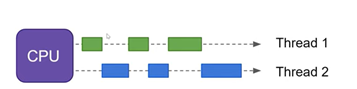
The lseg.data Python library is the gateway into LSEG's data environment. To begin retrieving content, you must first establish connectivity and authentication to the data environment. LSEG provides access to content either from the desktop (Workspace) or directly from the cloud (Delivery Platform). In either case, it is assumed you have credentials to access LSEG content and have installed the Python data library in your environment.
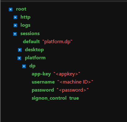
For manageability and flexibility, define your credentials in the lseg-data.config.json file.
# Session configuration outlined within lseg-data.config.json
ld.open_session()
Accessing portfolio content
The suite of services provided by PAM is broken down into logical sections:
- Metadata
Capabilities to retrieve metadata such as classifications, characteristics, asset classes, etc. - Analytics
The ability to run analysis on both user-defined portfolios and market indices. - Portfolio
Retrieve portfolio details including searching for portfolios and listing header values.
When performing basic analysis, users are required to provide a key element called the Portfolio ID, which identifies the specific user-defined portfolio or market index they wish to analyze. Users who are experienced working with LSEG portfolios are familiar with the Workspace apps: PAL (Portfolio and Lists Manager) and PORTF (Portfolio Analytics). These apps are tightly integrated, allowing users to easily select the portfolios they wish to analyze. However, when working with PAM, users must obtain the Portfolio ID. The challenge is that Workspace apps do not expose the Portfolio ID, so obtaining it requires interrogation and searching using a combination of Workspace and PAM APIs.
The following examples outline common mechanisms for users to locate the IDs they may need in their workflows.
Portfolio Finder
The PortfolioFinder is a simple, convenient tool allowing users of PAM APIs the ability to identify a specific ID required for purpose of analyzing portfolios. This GUI-based tool provides the ability to sort and filter content for ease of selection. For example:
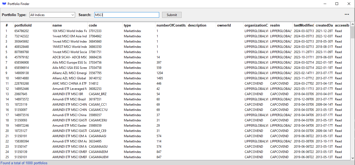
The primary purpose of the utility is the display of the portfolioid column. This ID is the driving key for the usage of the PAM APIs, allowing users to pull up metrics and portfolio details required for analysis.
While this utility does allow for a simple and effective way to interrogate the portfolio service to access the required portfolio IDs, users may prefer a programmatic mechanism to interrogate and select the portfolios for their specific work-flow. As part of the PAM APIs, a specific portfolio search capability is defined. The following examples outline what users can do with the APIs:
# The portfolio search function defines the mechanism to pull down the required IDs.
help(portfolios.search)
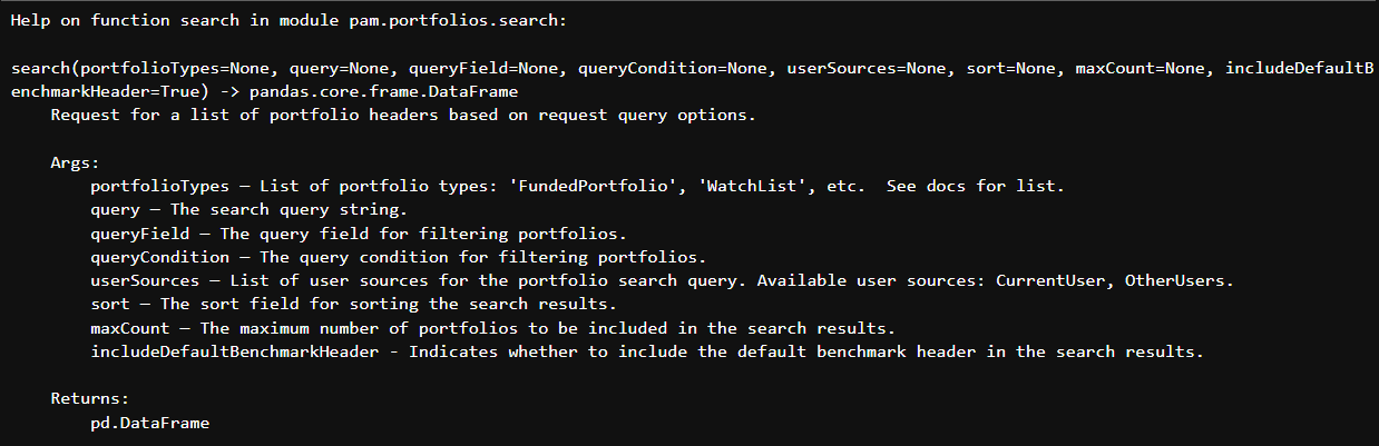
The Portfolio Type drives the main selection of the portfolios of interest. Here is a brief explanation of the types:
- FundedPortfolio
A set of Holdings Statements that represent the holdings of a portfolio over time. A Holdings Statement is a list of securities, their position amounts (e.g. shares, Par value, etc.) and costs on a particular date. - CompositeFundedPortfolio
A weighted portfolio containing other portfolios or benchmarks. For example, you can use this portfolio type to create a custom benchmark with 50% FT 350 and 50% Barclays Aggregates - WatchList
Simple list of securities with no weights or holdings. - MarketIndex
Representing Indices and benchmarks (S&P, MSCI, etc). - CarveOutPortfolio
A portfolio based on a filter or ‘slice’ of an existing portfolio or benchmark and focused on a specific sector or classification. For example, you could pick FTSE AllShare as a base portfolio and exclude/include all the securities in Consumer Discretionary. - ModelPortfolio
Similar to a FundedPortfolio, but position amounts are specified as weights (e.g. percentages) rather that shares, etc.. - PeerList
A List of peers of an instrument. For example, a new peer list gets created when you go to a company page -> peer list and add another company to the default list of peers. - MonitorList
Similar to a WatchList, a list of instruments created in Monitor app
User-defined portfolios
Users will undoubtely need to analyze the portfolios they create. Whether its just a few or many dozens, the search facilitly does provide a way to pull down all or filter out specific ones of interest.
# Pull down all user-defined portfolios.
# The 'portfolioTypes' specifier is conveniently defaulted to all user-defined types
portfolios.search()
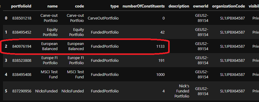
In the above display, I created a few test portfolios that are easily visualized and allow me to refer to the specific portfolioId of interest, as shown in the first column. However, depending on the number of user-defined portfolios you manage, further interrogation may be required to narrow down the ones of interest. With search, you can narrow your collection based on either the name or code fields. To filter portfolios containing "test" in the name or code, you can do the following:
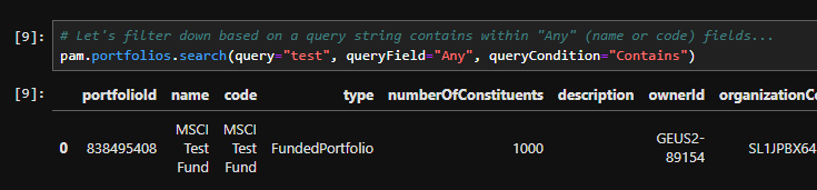
# Let's filter down based on a query string contains within "Any" (name or code) fields...
portfolios.search(query="test", queryField="Any", queryCondition="Contains")
Index Portfolios
Depending on entitlements, users may have access to thousands of system-defined indices that act as benchmarks and can be used to derive composite portfolios. In the above output, there are two key columns of data, name and code. When searching for portfolios, the API allows users to filter results by one or both of these fields.
®The number of indices available is extremely large, and requesting the entire data set will likely time out. Retrieving thousands of results is difficult to navigate and often unmanageable. This service is designed to filter the result set, allowing users to narrow down portfolios of interest. By specifying precise queries, users will reduce execution time and obtain more manageable results..
For this analysis, I plan to choose a benchmark of interest for comparison. Specifically, I'm going to look for an Intercontinental Exchange (ICE) index. You will likely need to be quite specific in your request to narrow down the index of interest.
# The 'portfolioTypes' specifier is required to ensure you are searching for index-based portfolios
portfolios.search(portfolioTypes="MarketIndex",
query="ICE BofA Global High Yield European",
queryField="Name",
queryCondition="Contains")
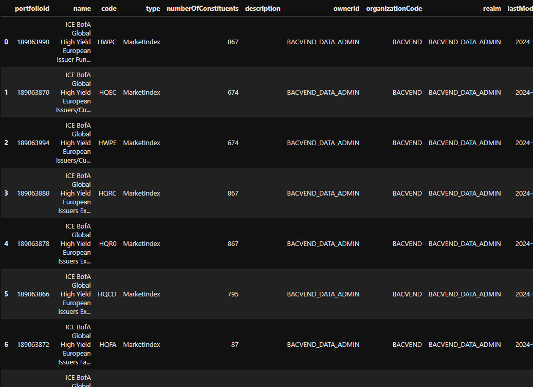
The query I used above was developed through experimentation. I started with a basic search and, as expected, more than a thousand portfolios were returned. I refined the query until it produced a reasonable, manageable result set and then selected the specific benchmark portfolio for this example.
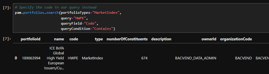
More experienced users can use the code field, which is more specific and, if known, can help narrow results. For example, I know a benchmark with the code 'HWPE'. Using that code, I can request the portfolio as follows:
# Specify the code in our query instead
portfolios.search(portfolioTypes="MarketIndex",
query="HWPE",
queryField="Code",
queryCondition="Contains")
From here, I can continue the same trend to narrow down portfolios of interest. For example, below are 2 benchmark portfolios I wish to compare against. For this task, I've chosen to use the PortfolioFinder utility as I simply need to identify the ID to perform my analysis.
In the first case, I'm performing a query based on an assumption of the name of the index:
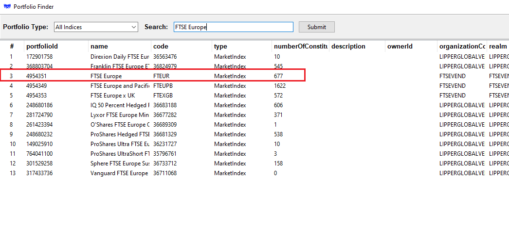
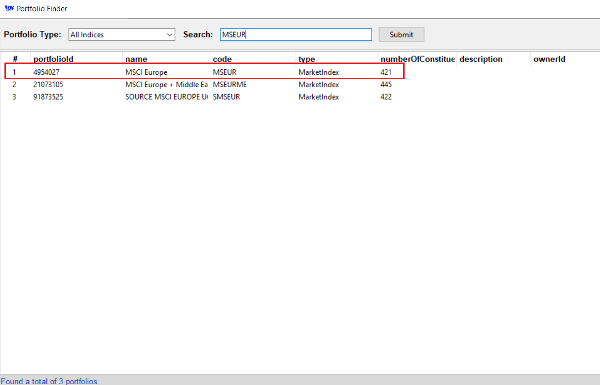
Next, I happen to know the code for the portfolio and will give that a shot:
Portfolio Charts
Once we have successfully narrowed down the portfolios of interest, we can demonstrate some of the value-add capabilities available in PAM. For example, within Workspace PORTF, when charting portfolios, users are limited to a fixed monthly frequency. While that representation provides a general overview, users may require more granular reporting.
The following examples demonstrate how to retrieve portfolio attribution measures and chart these metrics at daily and weekly frequencies.
To support these requirements, I have set up a couple of convenient functions that will aid extraction and presentation.
Step 1 - Data generation definition
The following function contains a code segment that defines the request to retrieve portfolio attribution measures and captures the results used for report generation. Step 3 below demonstrates how to generate the data.
# Define the core request to retrieve performance attributes
query_payload = {
"analysisDateRange": {},
"baseCurrency": "USD",
"portfolioOptions": {
# Programmatically assign our portoflio ID: "portfolioId": id,
},
"cashHandlingOptions": {},
}
# The portfolio attribution measures generation function supports the specification
# of multiple portfolios.
def generate_data(ids, start_date, end_date):
# Ensure the portfolios data is a list
if isinstance(ids, str):
ids = [ids]
query_payload["analysisDateRange"]["startDate"] = start_date
query_payload["analysisDateRange"]["endDate"] = end_date
# Step 1 - retrieve the portfolio labels/names
portfolios = pam.portfolios.get_portfolios(ids)
# Step 2 - retrieve daily statistics
df_result = pd.DataFrame()
for id in tqdm(ids):
# ID we're analyzing
query_payload["portfolioOptions"]["portfolioId"] = id
# Retrieve data...
performance = pam.analytics.get_performance_attribution(query_payload)
# Organize the data
df = performance.dailyCumulative[['date','portfolioCumulativeReturn']]
# Provide a friendly label for this data set
df = df.rename(columns={'portfolioCumulativeReturn':portfolios.headers.loc[id]["name"]})
# Collect the data
if df_result.empty:
df_result = df
else:
df_result = pd.merge(df_result, df, on ="date")
# Ensure our time scale is the a date-only index
df_result['date'] = pd.to_datetime(df_result['date'])
df_result.set_index('date', inplace=True)
print("Done")
return df_result
Step 2 - Data visualization definition
Once the data has been successfully generated, we can perform a simple visualization of the results. The chart_data function uses the Plotly Express package to plot our data, providing interactive hover information and optional brushing over data points to inspect values.
def chart_data(data):
fig = px.line(data, height=600)
# Update layout to move the legend inside the plot area
fig.update_layout(
title='Portfolio Analysis',
plot_bgcolor='black', # Change plot background color to black
paper_bgcolor='black', # Change paper (entire figure) background color to black
legend_title_text='',
legend=dict(
x=0, # x position of top-left corner of legend
y=1, # y position of top-left corner of legend
bgcolor="rgba(0, 0, 0, 0)", # semi-transparent white background
bordercolor="white",
borderwidth=0
),
font=dict(color='white') # Change font color to white
)
fig.update_yaxes(tickfont=dict(size=10), gridwidth=0.1, gridcolor='grey', title_text="returns")
fig.update_xaxes(gridwidth=0.1, gridcolor='grey') # Adjust the x grid lines
pio.renderers.default = 'png'
fig.show()
Step 3 - Generate and plot
Putting it all together, we can now generate the portfolio attribution measures for our portfolio(s) and chart the results.
# Example 1 - generate measures for our user-defined portfolio referenced as 'European Balanced'.
# The date is based on the portfolio we created
df = generate_data("840976194", "2022-07-31", "2025-10-31")
# Then chart the results...
chart_data(df)
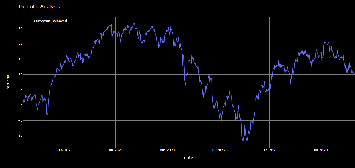
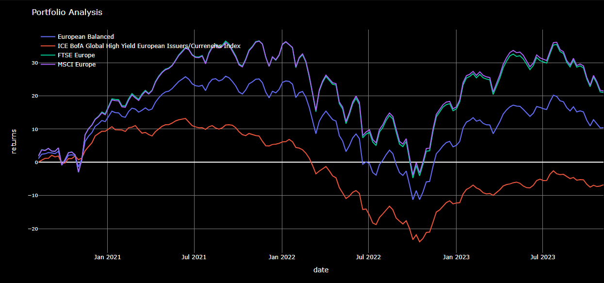
While the above chart can be generated within the Workspace PORTF application, the goal here was to demonstrate the basics of charting programmatically. With the basics in place, we can move on to something a little more interesting — comparing our 'European Balanced' portfolio to the benchmarks shown above.
# Example 2 - Include the following benchmark indicies for the comparitive analysis:
#
df = generate_data(
["840976194", # European Balanced
"189063994", # HWPE - ICE BofA Global High Yield
"4954351", # FTSE Europe
"4954027"], # MSCI Europe
"2022-07-31", "2025-10-31" )
# Then chart the results...
chart_data(df)
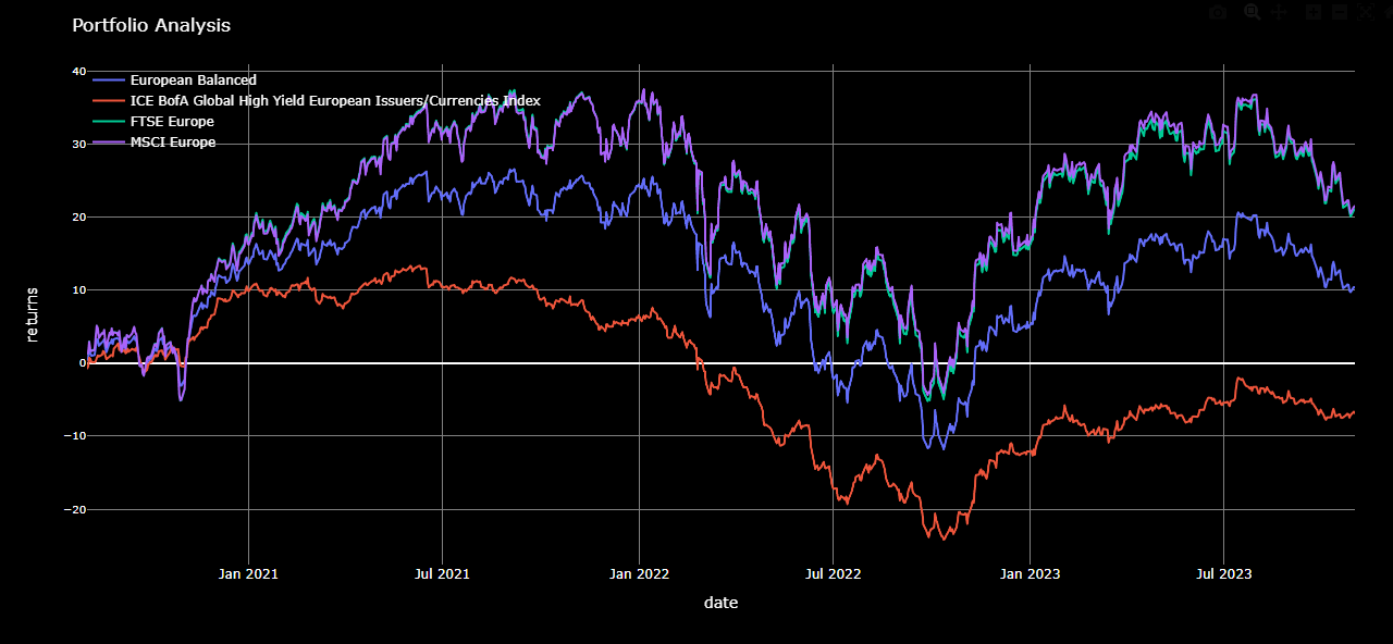
By default, the data returned from our portfolio backend contains daily measures across the specified timeframe. From our results, the above chart was produced based on these daily measures. However, we can manipulate the data to present the granularity in any timeframe of our choosing.
# Weekly
df2 = df.resample('W').mean()
chart_data(df2)
Summary
Working with GUI-based desktop applications will always be a powerful mechanism for easy and rapid analysis. Their intuitive interfaces and comprehensive capabilities provide users with immediate insights into their portfolios. However, these applications, despite their ease-of-use and quick analytical abilities, are not without limitations. Exposing the inner capabilities of portfolio analysis through their APIs empowers the user to customize, extend, and integrate portfolio data into their workflows seamlessly. Providing users with the underlying data allows the flexibility of accessing and presenting the results within their own applications. While this article does touch on a very simple subset of the capabilities available, users are encouraged to explore the wealth of PAM APIs to discover the full potential of their data for comprehensive analysis and decision-making.
- Register or Log in to applaud this article
- Let the author know how much this article helped you