

| New to the series? Start with the Series Index for setup, scope, and context. |
You've opened a session. You've made your first call. Now it's time to write code that's reliable, readble, and easy to build on.
This volume is about the patterns that sit underneath almost everything else you'll do with the library - the details that make the difference between a request that works and a request you understand. Date logic, parameter placement, field propagation, column naming, debugging, and a few shortcuts that quietly save hours.
These aren't advanced topics. They're foundational ones. The developers who pick them up early spend less time second-guessing their requests and more time doing something interesting with the data they return.
| Table of Contents |
|
Snapshot or Series
| 💡Picking the right call before you write it |
The library gives you two primary calls. Knowing which one to reach for before you write the request is what keeps your output shaped the way you expect.
- get_data() - returns a snapshot. Latest or reported value. One row per instrument by default.
- get_history() - returns a time series across a date range. One row per period, indexed by date.
The key distinction is the primary axis:
get_data() is instrument-first. get_history() is time-first.

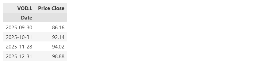
Things to keep in mind
SDate/EDate in get_data() retrieves values across a period - it doesn't produce a time series. The result stays instrument-first: you'll get a RangeIndex, not a DatetimeIndex. When you need a genuine time-indexed series, get_history() is the right call.
Some TR.* fields are designed for get_data(), not get_history(). Fundamental and point-in-time fields aren't stored as native historical time series on the backend. For these, get_data() with SDate, EDate parameters is the correct and intended approach - not a workaround.
Inline vs. Global Parameters
| 💡Place a setting where it actually belongs |
The choice between inline and global parameters comes down to one question: do all your fields need the same setting?
Global parameters - one setting, all fields
Pass a single parameters dictionary and every field in the request picks it up. Fields that don't support a given global parameter simply ignore it - cleanly, with no error and no side effect.

Inline Parameters - Different Settings Per Field
Embed the parameter directly inside the field string. This is the only way to retrieve the same field multiple times with different settings in a single request.

Mixing Them
Global sets the default. Inline overrides it for a specific field.

Things to keep in mind
There's a deliberate asymmetry worth knowing: a global parameter that a field doesn't support is silently ignored. The same unsupported parameter supplied inline raises an error. Same parameter - different behaviour depending on where it lives.
This is actually useful: the inline error is immediate feedback that something is mismatched. Check supported parameters in the DIB before going inline and you'll never hit it unexpectedly.
Field Propagation
| 💡Get metadata without a second call |
A value is more useful with its context. "TR.Revenue" is far more meaningful when you also know the reported date, the reporting period, and the currency it was filed in. Field propagation gives you all of that in the same call - no extra requests, no manual alignment.

Each propagated attribute returns its own column, aligned with the parent value automatically.
Propagation Respects Inline Parameters
A propagated attribute follows the parameterised version of the field it hangs off. Request the same field at multiple periods, and each .date returns the date for its own parent - not a shared default.

Each ".date" is bound to its specific parent. Three field requests, three distinct dates.
Things to keep in mind
Some attributes track your Parameters. Some track the Filing and other details. This distinction is where propagation really pays off.
The below example using Currency makes it clear:

- ".currency" reflects your curn - the INR you converted to.
- ".companycurrency" reflects the company's native reporting currency - a fact about the filing, not your request.
Supported propagating attributes vary by field. To see what's available for a given field, open it in DIB → Parameters → Output. If a field doesn't support propagation, request the metadata field separately.
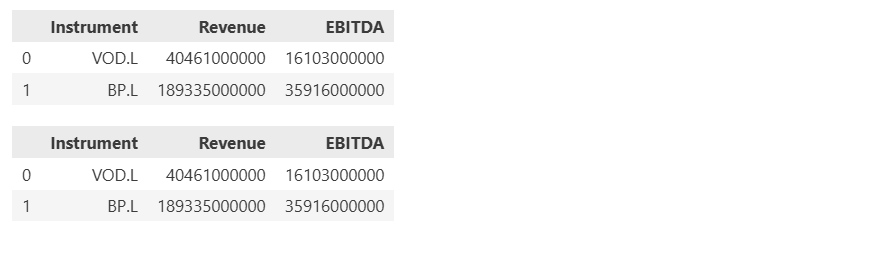
Rule of thumb:
Use lists in production code. They're easier to build programmatically, more readable.
The semicolon form is genuinely handy for quick experiments - less typing, easy to paste from a config or user input. Personally, it's the one I reach for when I'm still working out what I want to ask.
Machine-Friendly Column Headers
| 💡Column names built for code, not just reading |
By default, the library returns human-readable column names - e.g. "Price Close". These are great for reports and notebooks you're sharing. For code that processes the data programmatically, you want names that are stable, deterministic, and unambiguous.
"header_type" gives you full control:

Available options:
| Option | Output | Best for |
|---|---|---|
| ld.HeaderType.TITLE | Price Close - human-readable (default) | End-user reports |
| ld.HeaderType.NAME | TR.PriceClose - stable and deterministic | Production code, pipelines |
| ld.HeaderType.NAME_AND_TITLE | TR.PriceClose | Price Close | Shared notebooks where both matter |
NAME is especially valuable when requesting the same field multiple times with different inline parameters - it's the only way to get columns you can reliably tell apart.
Debugging and Logging
| 💡Seeing what the library is actually doing |
When the surface error isn't enough, debug logging is the fastest route to an answer. It shows you exactly what the library is sending and receiving - and it's the first thing support teams and community moderators will ask for when helping you troubleshoot.
Two ways to enable it:
Method 1 - Configuration File
Add a "logs" section to your config file. The library picks it up automatically at startup.
Method 2 - Programmatic Configuration
Set params in code before opening your session - no file edits needed.
Both methods are equivalent - pick whichever fits your workflow.
Things to keep in mind
Debug logging is a diagnostic tool - turn it on to investigate, turn it off when you're done. Leaving it running in long-running production workloads generates large log files and may capture request details you don't need to retain.
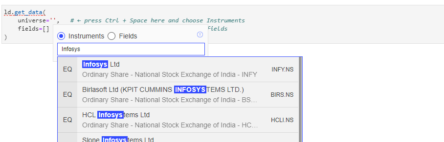
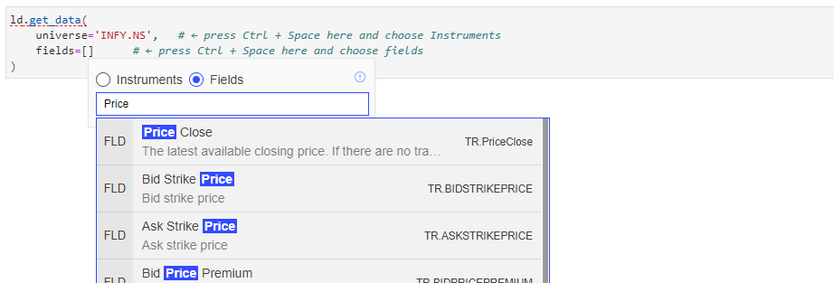
Inline search - inline results - no context switch. Particularly useful when exploring unfamiliar content sets or verifying field names before committing to them.
Things to keep in mind
This is a CodeBook-native feature - it isn't available in VS Code, JupyterLab, or local Python environments. Outside CodeBook, the Data Item Browser is the closest equivalent and covers the same ground.
Ctrl+Shift+Space
| 💡Use LSEG Workspace search from anywhere |
If Workspace is running on your desktop, "Ctrl+Shift+Space" opens the global Workspace search bar without switching applications. Useful mid-flow when you need to verify an identifier or locate an instrument reference without breaking your train of thought.
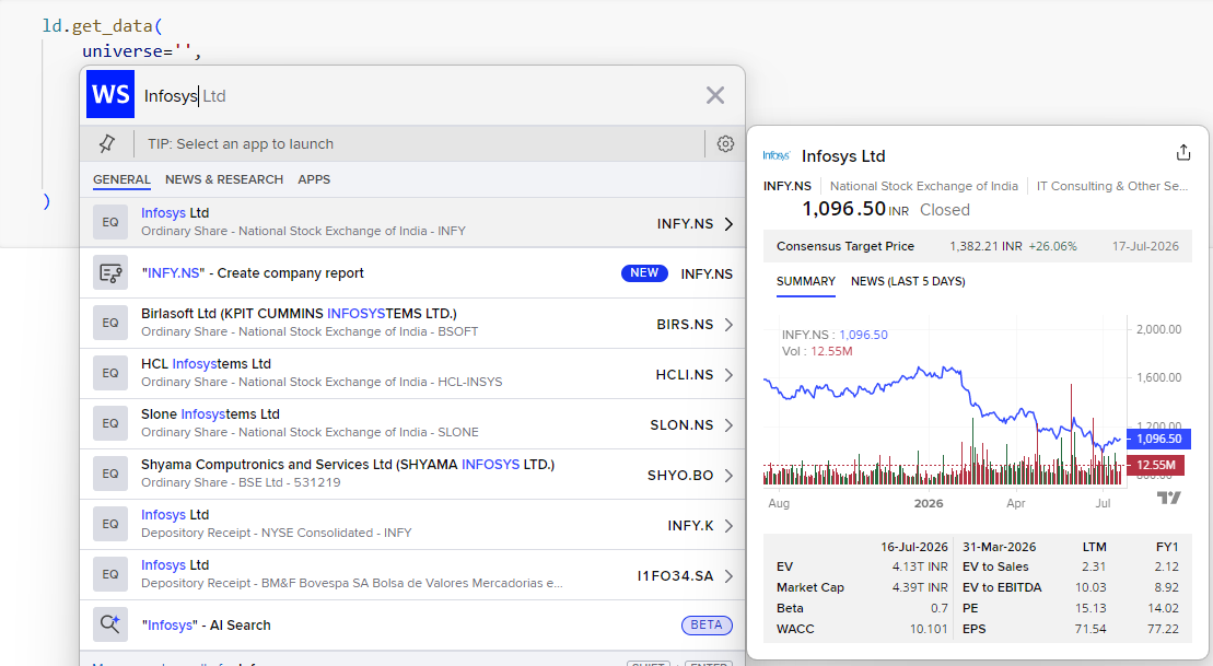
Things to keep in mind
This shortcut works with a desktop Workspace session - Workspace must already be running on the machine. It isn't relevant when connecting through a Platform Session.
That's Your Foundation
Every pattern in this volume sits underneath something bigger. Parameter placement, field propagation, column naming - these are the mechanics that make every other capability in the library easier to use, debug, and build on.
You now have what you need to write requests you can trust: calls that return the right shape of data, with the right context, in a form that's ready for code. The rest of the series builds from here - relative dates, embedded calculations, async requests, and more.
Up Next:
| ← Series Index | Vol. 2 Asking What You Mean → (Write requests that bring data exactly what you meant) |
- Register or Log in to applaud this article
- Let the author know how much this article helped you

Related APIs
In This Series
Related Articles
-
Check LSEG Data Library for Python Usage Limits Remaining
-
The Data Library for Python - Quick Reference Guide (Access layer)
-
Step-By-Step Guide to install Data Library for Python using Virtual Environment
-
LSEG Data Library for Python: News Pagination
-
LSEG’s Refinitiv Data Library for Python and its Configuration Process