
Article
Integrating Julia and Python for Seamless Financial Data Retrieval

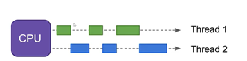
In the field of data analysis, when it comes to choosing the right technology and programming languages, Python, with its extensive set of libraries and powerful syntax, has become the cornerstone for data scientists worldwide. It’s not just a language; it’s a comprehensive toolkit that has transformed the landscape of data analysis, making it a popular choice for professionals in the field. Yet, there’s another language making its presence felt in the data science community: Julia. With its user-friendly syntax and impressive performance, Julia is steadily gaining recognition and is proving to be a noteworthy alternative in the field. Julia has been gaining popularity for its speed and user-friendly syntax. As of 2021, Julia had been downloaded over 40 million times, indicating a growing interest in the language.
One of Julia’s key strengths is its speed, comparable to languages like C and Fortran. This makes Julia particularly useful for high-performance computing. Additionally, Julia’s syntax is similar to that of Python and MATLAB, making it an easy transition for programmers familiar with these languages. While acknowledging that Python currently boasts a comprehensive set of packages, some of which may not yet be available to the Julia community, it is important to consider the evolving landscape of both programming ecosystems. To help gain access to more capabilities and data, the Julia community includes a popular and powerful package to bridge access to the Python landscape.
In this article, we explore how to use Python packages in Julia, focusing on retrieving company financial data within the Jupyter environment. We’ll demonstrate how Julia and Python can work together to perform sophisticated data analysis tasks.
For more on Julia’s rise in popularity, you can refer to articles such as The Rise of Julia — Is it Worth Learning in 2023? and Why We Use Julia, 10 Years Later.
Getting Started
For this analysis, the following components will be required to execute the source code available within this article.
- Python
- Refinitiv Data Library for Python
The component that provides access to LSEGs financial data. Note: Users are required to have access credentials to retrieve data. More details are provided in the section below. - Jupyter (lab or notebook)
- Refinitiv Data Library for Python
- Julia
- Julia Packages
A number of packages including PyCall and IJulia to enable access to Python packages running in a Julia kernel within the Jupyter environment
- Julia Packages
When working with Python, users have many choices and options to setup their environment. Users can drive their setup by installing Julia then going through the steps to setup Jupyter within a conda environment. However, this article doesn't focus on the different installation options but rather the basic components used and general instructions based on my current setup. For example, I have an existing Python and Jupyter lab setup within my environment that includes the Refinitiv Data Library for Python accessing financial data. Given this, I will walk through the basic steps to add the Julia environment to the existing Python setup:
- Download and install Julia
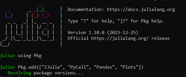
- Add the required Julia packages:
- IJulia (Jupyter Kernel)
- PyCall (package to bridge calls between Julia and Python)
- Pandas (Working with Pandas DataFrames)
- Plots (Charts)
Once Julia has been download, follow the instructions in the above link to install. Once installed, you can begin the process of adding the required packages and setting up the IJulia kernel within Jupyter.
On the command line, launch the Julia interactive command-line interface REPL:
> julia
Once launched, you can begin to install and setup the package environment within Julia:
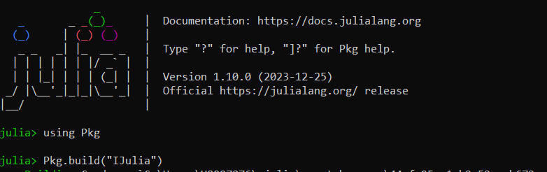
Once the required Julia packages have been downloaded, some packages require a further build step. The build step performs tasks such as compiling the package necessary for operation. For example:
- IJulia - Build required to set up the Julia kernel for Jupyter Notebooks
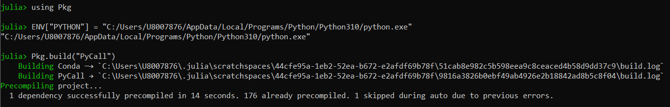
- PyCall - Build required to set up the interface between Julia and Python
Below, you will need to setup your environment prior to building the next package. The 'PyCall' package requires knowledge of your Python environment during the build phase. By default, when attempting to build the PyCall package, it will attempt to use a Conda package. However, in my case, I have an existing Python installation, so I will need to notify Julia where this is by setting the following within Julia:
As the final setup step, install the Julia kernel for Jupyter. This is a one-time setup that allows you to seamlessly use Julia within the Jupyter environment.
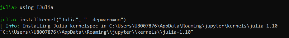
Once completed, you can exit out of the Julia command-line utility (^d) and confirm whether the IJulia kernel has been successfully installed within your Jupyter environment:
> jupyter kernelspec list
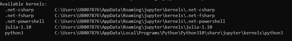
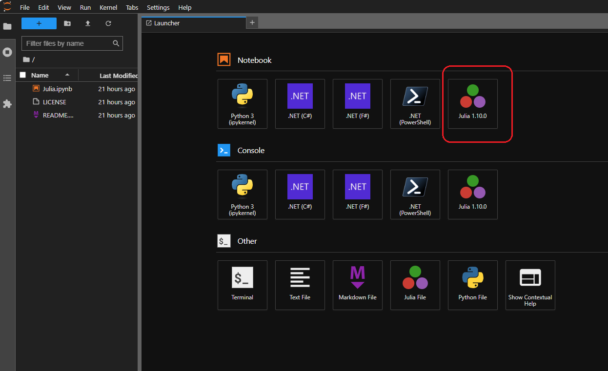
Among the available kernels, you should see an entry for Julia. At this point, you can launch your Jupyter environment:
# Launch Jupyter
> jupyter lab
Working with Financial Data
The following examples are defined within the example notebook providing popular data retrieval examples with simple and complex presentation. The goal is to show how to leverage the power of your Python packages within Julia by accessing the wealth of content and financial data available from LSEG.
Let's start by setting up your Julia packages:
# PyCall - Provides the ability to directly call and interoperate with Python
using PyCall
# Julia interface to the Python library 'pandas' managing dataframes received from LSEG data services
using Pandas
# General Julia packages
using Dates
using Plots
# Import the Python libraries we plan to use...
rd = pyimport("refinitiv.data") # Data Library for Python
pd = pyimport("pandas") # Pandas library - used to perform calculations
Open a Session to access data
The refinitiv.data Python library is the gateway into LSEG's data environment. In order to begin the retrieval of content, you must first establish connectivity and authentication within the data environment. LSEG provides access to content within either the desktop (Workspace) or platform (RDP) environments. In either case, it is assumed you have credentials to access content from LSEG and have utilized the Python data library within your own Python environment.
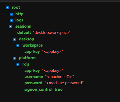
For management and flexibility, it is easiest to define your credentials within the 'refinitiv-data.config.json' file.
# Open a session into the data platform
# Ensure you have defined your access credentials within the 'refinitiv-data.config.json' file.
session = rd.open_session()
PyObject
Throughout the use of the PyCall interfaces, a user-defined object of type 'PyObject' will be returned from each call. The PyObject acts as a bridge between Julia and Python that will intelligently provide access to the underlying Python interfaces. You can actually observe the underlying Python type using a convenient PyCall function.
# Return the underlying Python object.
pytypeof(session)
PyObject <class 'refinitiv.data._core.session._platform_session.PlatformSession'>
Data Access
At this point, you can begin your regular data access calls as if you are within Python, passing parameters within method calls. However, there will be some slight differences working with the data when accessing content that I will point out as we walk through some examples. I will also demonstrate how you can work with other Julia packages by bridging the data that is returned from Python.
Search
LSEG provides a comprehensive data service offering the ability to search a wide range of content such as quotes, instruments, organizations, etc. Many of the data services available from LSEG require key codes such as RICs, ISIN, CUSIPs to pull down key datasets including historical values and company fundamentals. The Search service is a powerful way to capture these key codes based on google-like query expressions and powerful filtering rules and conditions. For more details, refer to the Building Search into your Application Workflow article.
# Search - Retrieve instruments with the ticket 'vod', a coupon of 5% and maturing in 2025.
response = rd.discovery.search(
query="vod 5% 2025",
select = "CouponCurrency, CouponTypeDescription, IssuerLegalName, CouponRate, MaturityDate, ISIN"
)
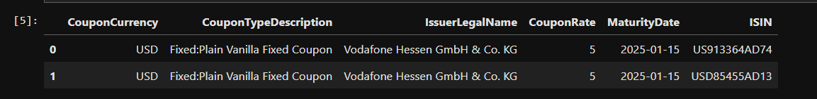
While the above execution is done entirely within Julia, users who are familiar with this library should also observe that the syntax is seamless for Python developers. This is the advantage of the PyCall library and how seamless execution can occur. In addition the user is presented with a tabular result appearing very much like what you would expect within an IPython kernel. However, because we are in IJulia, the object itself is a PyObject that acts a bridge to an underlying Pandas DataFrame within Python.
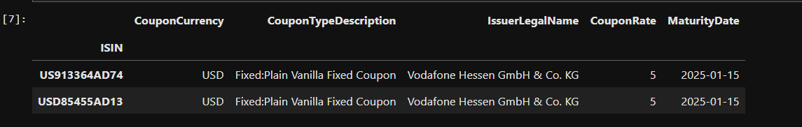
To demonstrate how we can work with the underlying Dataframe from Julia, let's try performing some activity on the result.
# Change the index of the dataframe.
df1 = response.set_index("ISIN")
As you continue to progress with your application execution, it may be preferable to work with Julia-based packages as opposed to the Python bridging access. For example, below I'm utilizing the popular Julia-based Pandas package to convert my PyObject-based Pandas Dataframe.
# Let's work envirely within Julia instead by utilizing the DataFrame Julia-based package.
df2 = DataFrame(response)
# Let's show what we're working with...
typeof(df2)
DataFrame
# And some basic data access using the Julia DataFrame
df2["ISIN"][1]
"US913364AD74"
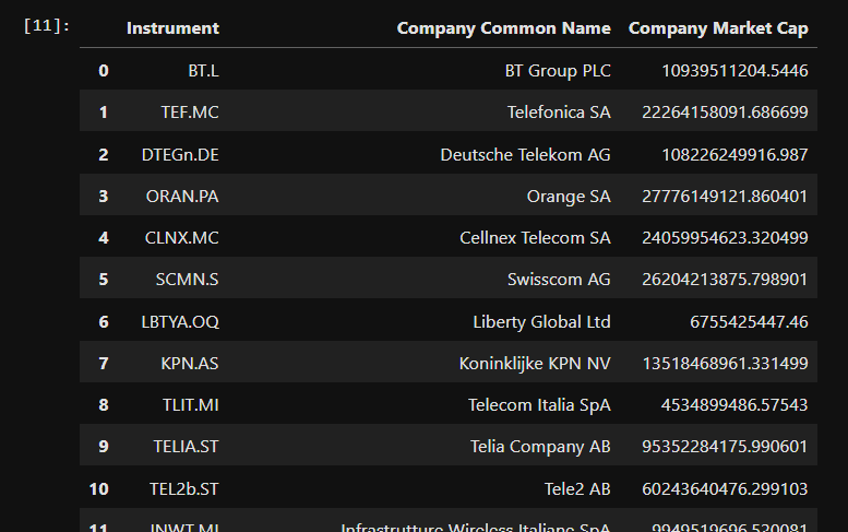
get_data
To demonstrate some other popular capabilities users rely on when working with the LSEG Python Data Library - the ability to access company data and fundamentals.
# get_data()
response = rd.get_data("Peers(VOD.L)", ["TR.CommonName", "TR.CompanyMarketCap"])
Historical Pricing
In this example, I'll apply a number of features that demonstrates the manipulation and charting of historical market data. Based on the Simplifying Intra-day Market Analysis: article, I will extract, manipulate and chart Intra-day historical data points. The goal is to walk through a more complex example that showcases working with Python DataFrames and charting features.
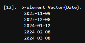
# Step 1 - extract the last 5 dates (monthly) from the USDA World Agricultural Supply and Demand Estimates
response = rd.get_history("C-CROP-ENDM0")
dates = [Dates.Date(dt) for dt in response.index][end-4:end]
# Step 2 - Iterate through our dates and retrieve the historical intraday measures.
# For each data set, perform some basic calculations to prepare the results.
prices = []
#pd.set_option("future.no_silent_downcasting", true) # Uncomment is you see downcasting warnings
for dt in dates
result = rd.get_history(
"Cv1", # Corn
["TRDPRC_1", "ACVOL_UNS"],
"1min",
"$(DateTime(dt, Time(15, 21, 0)))",
"$(DateTime(dt, Time(21, 51, 0)))")
df = result.dropna()
df = df.tz_localize("UTC")
# Convert the date index for local time (nice for presentation)
index = df.index.tz_convert("America/Chicago")
df = df.set_index(index)
# Ensure our valies are numeric and calculate our net measure...
df["TRDPRC_1"] = pd.to_numeric(df.iloc(1)[1])
df["TRDPRC_1"] = df["TRDPRC_1"] - df["TRDPRC_1"].iloc[1]
price_df = df.drop(["ACVOL_UNS"], axis=1)
price_df.rename(columns=Dict("TRDPRC_1" => Date(price_df.index.max())), inplace=true)
price_df.index = price_df.index.time
# Keep track of each dataset
push!(prices, price_df)
end
# Step 3 - Combine the extracted prices (dataframes) and place them within our data object
data = pd.concat(prices, axis=1, sort=false).dropna()
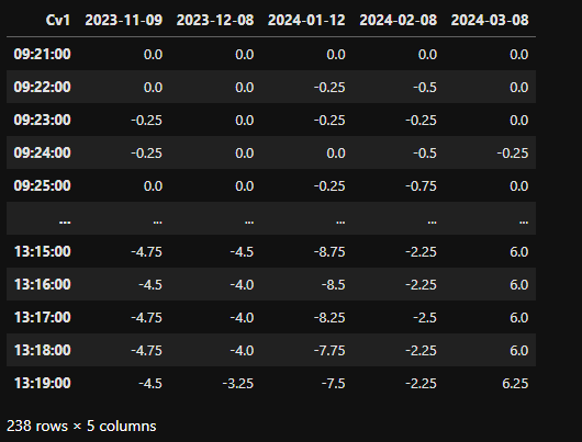
# Step 4 - Now that we have pulled down the raw data measures, let's convert the data
julia_data = DataFrame(data)
show(julia_data)
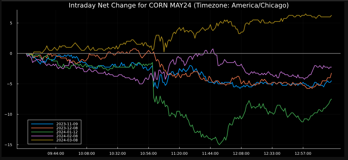
# Step 5 - Prepare and chart our measures...
# Set the plot size
default(size = (1100, 500))
# Pull out the index representing the x-axis - array of PyObjects
idx = collect(index(julia_data))
# Create an array of Julia DateTime objects from the index
julia_datetime_array = [DateTime(2000, 1, 1, getproperty(tm, :hour), getproperty(tm, :minute), getproperty(tm, :second)) for tm in idx]
# Format DateTime objects as HH:MM:SS
times = [Dates.format(dt, "HH:MM:SS") for dt in julia_datetime_array]
# Retrieve the data points...
data = [Array(julia_data[name]) for name in columns(julia_data)]
# Extract the column names
column_names = collect(columns(julia_data))
# Start with a fresh plot
p = Plots.plot()
title = "Intraday Net Change for CORN MAY24 (Timezone: America/Chicago)"
# Plot each line separately with its corresponding label
for (i, column) in enumerate(column_names)
plot!(times, data[i], label=column, lw=2)
end
title!(title)
# Customize the plot
plot!(background_color = :black, foreground_color = :white)
# Add a horizontal line at zero
hline!([0], color=:grey, linewidth=2, label="")
Realtime Pricing
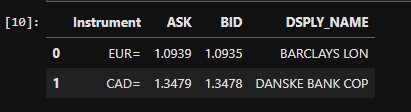
As our final example, I will utilize the streaming pricing interfaces available from LSEG to demonstrate working with real-time data by utilizing a common feature available within the Python library. With this example, I will subscribe to a set of instruments that populate a live cache. At any point, you can programmatically pull out real-time data from the cache on an on-demand basis.
# Subscribe to a few instruments and some relevant fields.
# This done by creating a stream definition...
stream = rd.open_pricing_stream(
universe=["EUR=", "CAD="],
fields=["DSPLY_NAME", "BID", "ASK"]
)
# Open the stream...
stream.open()
At this point, we have opened a subscription to capture live data points from the registered instruments: Euro and the Canadian Dollar. This specific action has populated our internal cache with real-time values. Let's view the cache:
# Retrieve and display realtime pricing cache...
stream.get_snapshot()
Because our subscriptions are open, we have a live cache that is updating based on changes in the market. At any point, you can pull down the cache and view the latest values.
stream.get_snapshot()

After short period, we can see the changes in our cache based on the changes in the market.
Observations
It's clear the immediate benefits having access to existing capabilities within Python and the wealth of packages available. The PyCall interface does a fantastic job of seamlessly bridging Julia and Python to make developers feel at home in both languages. Coupled with the Pandas package, accessing content within the LSEGs Financial data library for Python is clearly a quick win. During my journey, I did come across a few roadblocks that other Julia developers may stumble on, such as attempting to work with the DataFrame Julia package. While I was able to figure out how to bring in a Pandas DataFrame into a native Julia DataFrame package, it was at a cost of extra processing and work. Users that do prefer to work with native Julia-based DataFrame objects from the DataFrames package will have to consider the challenges. While I found success in the above examples, I did not perform a comprehensive analysis of all capabilities and expected operation of the library. For example, I believe there may be challenges when registering callback functions within the library and whether this is a cumbersome action or potential roadblock for developers. While I am in favor of a native Julia package that provides clean and expected integration, having the immediate power of accessing services and resources through the Python ecosystem is powerful tool.
- Register or Log in to applaud this article
- Let the author know how much this article helped you