This formula is a simplified approach, evaluating risk by using depth as a proxy for risk attenuation scaled by the probability of default for the common supply chain ancestor. It assumes that greater distance from the ancestor default allows the chain to absorb defaults (represented in the exponential decay in the e term); however, it is worth noting that it is possible that the bullwhip effect actually exacerbates the risk implications. Additionally, this formula does not consider factors such as the availability of substitute suppliers or potential response times. The decision to omit these considerations stems from their unpredictable nature, which would likely require a considerable machine learning solution to estimate reasonably.

Overall portfolio risk is evaluated as the sum of risks from all conflicts:

To illustrate the real world effectiveness of this approach, we will use the SPDR corporate bond portfolio as our diversification candidate. This portfolio has been rated 3 stars by Morningstar, indicating it is "fairly valued."

Imports

Starting off we import the necessary libraries. Here we use the LSEG Data Libraries to retrieve the data. The code is built using Python 3.9. We also define two variables used throughout the code here for simplicity. We also initialise our refinitive data sesssion.

Simulated SPBO Corporate Bond Portfolio

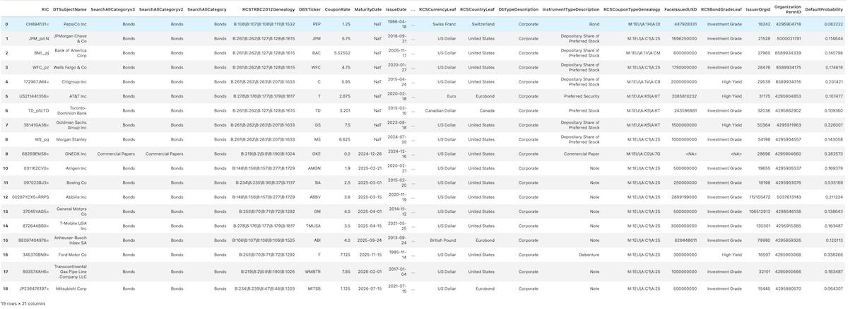
This portfolio is a simulation of the SPBO (S&P U.S. Corporate Bond Index) to demonstrate the real-world applicability of the proposed risk mitigation tool. Here we also migrate from identifying issuers with RICs to with their Organization Permanent IDs, this ensures that the companies themselves are evaluated, rather than the specified bond holdings - and privately traded companies can still be traversed through.

Attaching Default probabilities

As part of this process we also define a function to traverse a universe and return a dictionary of all associated default probabilities. Note that <NA> values are filled with the mean values.

Function Declarations for Value Chain Traversal

The following functions take a list of Permanent IDs for bond issuers in the original portfolio and generate a hierarchical tree of suppliers (or ancestors) within their respective value chains. The output is structured as a dictionary, where each key represents an organization ID, and its corresponding value is another dictionary containing its suppliers. This recursive structure, combined with constant-time lookup, enables efficient navigation and identification of common suppliers or value chain bottlenecks.

A queue-based approach is implemented in the API_call function to manage cases where a large universe of suppliers is requested. When an error occurs, the universe is recursively split into smaller subsets. This strategy is essential because the number of suppliers for each "head" is unknown, and the backend call could involve a significantly larger universe than initially anticipated, necessitating the breakdown of queries. A maximum retry attempt of two has been set, under the assumption that "bad" calls can occur, but they often happen consecutively due to specific problematic members of the "heads" list.

Generate Data Structure for Supply Chains

Execute the previously defined function traverse_value_chains to generate the supply chain data structure.

Processing 19 heads...
Finished layer 0 Traversal
Processing 95 heads...
Processing 96 heads...
Processing 100 heads...
Processing 100 heads...
Processing 98 heads...
Processing 40 heads...
Finished layer 1 Traversal

Weak Point Identification Function (Given Supply Chain Data Structure)

We define a recursive function to traverse the value chains using the provided supply chain data structure. Each unique organization is assigned a key in a lookup dictionary, termed loop_dict, where the value is a list of all bond issuers from the original portfolio that have this organization within their supply chain. This approach ensures an O(n) time complexity for traversing and analyzing the supply chain data.

Function: `isk_calc

The risk_calc function is designed to assess the risk associated with a bond portfolio by evaluating the contribution of individual portfolio constituents to overall risk, as well as the magnitude of specific conflict scenarios. 

Parameters:

- Supply_chains: A data structure representing the relationships between various entities in the supply chain, which can influence risk propagation.

- associated_portfolio: A Pandas DataFrame containing details about the bond portfolio, including organization identifiers and default probabilities.

Description:

This function performs the following key operations:

1. Conflict Identification: It identifies conflicts within the supply chain using the loop_identification function, which captures interdependencies between entities.

2. Pruning Conflicts: The function filters out non-relevant conflicts by retaining only those that meet a specified significant_conflict_size, ensuring that only meaningful conflicts are analyzed.

3. Risk Calculation:

   - For each identified conflict, it calculates the risk associated with each offender (i.e., portfolio constituent) by leveraging their default probability and a risk propagation model that includes an exponential decay factor based on the conflict's depth.

   - It aggregates the risks at both the individual offender level and the overall conflict level, providing a detailed score for each conflict.

4. Outputs:

   - The function returns three values:

     - total_risk: The cumulative risk for the entire bond portfolio.

     - individual_offender_scores: A dictionary containing the total risk attributed to each offender in the portfolio.

     - conflict_scores: A list of tuples, each containing a conflict identifier and its associated risk score.

Purpose:

This function serves as a vital tool for risk assessment in bond portfolios, using conflict supply chain depth as a proxy for risk propagation attenuation and leveraging default probabilities to inform risk metrics. It provides insights into the relative contributions of individual portfolio constituents to overall risk, allowing for informed decision-making and risk management strategies.

Generate Dictionary for Identified Weak Points and Corresponding Bonds

Execute the loop_identification function, followed by pruning the resulting dictionary to eliminate conflicts of significant magnitude.

Graph Example Points of Failure from Portfolio From Each Risk Level

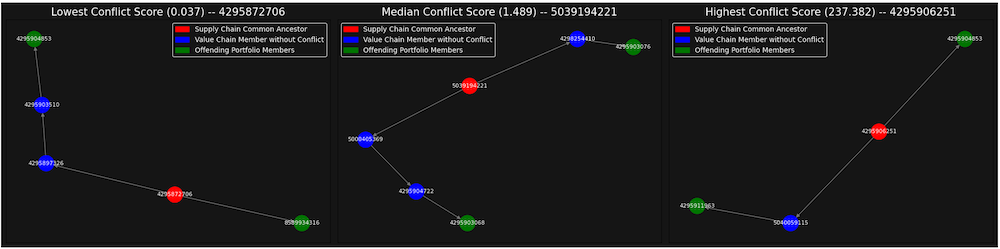
Using networkx and matplot we can visualise a given conflict quite easily. here we can contexualised relative constituents to risk by graphing the lowest risk collision, median risk collision and highest risk collision.

Split Portfolio into Remaining Bonds and Bonds to be Reselected

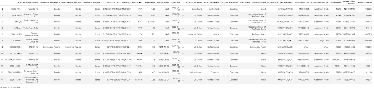
Using the individual offender scores, we can identify the largest contributors to overall portfolio risk and isolate the top offenders based on a specified percentage of the total risk we aim to eliminate. It’s important to note that attempting to eliminate all risk could result in selecting very small contributors, which might inadvertently introduce additional risk into the portfolio.

DataFrames of 'insecure' Bonds

DataFrame of 'Secure' Bonds

Query for Replacement Bond Suggestions

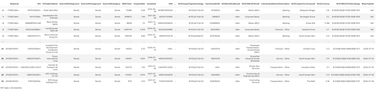
For each bond identified for replacement, candidate alternatives can be generated by querying the Refinitiv Data API. Filters will be applied to ensure that the replacement bonds align closely with the attributes of the original bond, including sector, coupon rate, and maturity date. This methodology establishes a targeted search space, consisting of a set of bonds, from which replacements can be selected to minimize supply chain conflicts.

Append 'Organization PermID' Column for Portfolio Optimization Methods

By appending each organization's Permanent ID (PermID) to the corresponding record, each bond can be uniquely indexed and efficiently queried. This step ensures that portfolio optimization methods can accurately track and analyze each issuer throughout the optimization process.

Resultant DataFrames

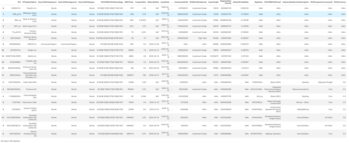
'Replacee' column denotes bond in original portfolio which is suggested to change. Each record then denotes the bond recommended as the replacement.

Traversing Replacement Candidates' Supply Chains

To optimize the selection of replacement bonds, it is essential to evaluate their supply chains in the same manner as the original bonds. The following code block performs this by traversing the suppliers of each candidate bond to generate its supply chain structure. This process ensures that the chosen replacement bonds will minimize conflicts with the existing portfolio.

Processing 84 heads...
Processing 78 heads...
Finished layer 0 Traversal
Processing 61 heads...
Finished layer 1 Traversal

Create Dictionary of Replacement Bonds

To facilitate efficient conflict testing and portfolio optimization, the replacement bonds are organized into a dictionary based on the 'replacee' RIC (Reference Identification Code) of the original bonds. This approach enables easy management and analysis of replacement options for each bond in the original portfolio.

Greedy Portfolio Optimisation Function Definitions

Here I provide a Greedy Portfolio Optimisation method. Individual solutions for different common ancestor depth categories are generated in decreasing order of risk (and therefore priority) - thereby ensuring that higher priority risks are resolved first. A greedy algorithm performs admirably in this context due to the limited scope of the search space (shallow supplier traversal depth). You could explore alternative optimisation methods - however, after trialling a genetic generation method, generated solutions severely underperformed in both generation time and risk reduction performance.

Generate the solution

Generate New Portfolio

Once the solution is generated using either the Greedy or Genetic Algorithm, it is used to update the portfolio. The generated replacement bonds are mapped to the previously created 'diversified' DataFrame, which uses the Perm OrganizationID as the index. This approach ensures that the replacement bonds are efficiently integrated into the new portfolio without the need to re-query the API.

Test Conflicts

Here we evaluate our diversified portfolio and compare to the original portfolio.

Old Portfolio Risk 1358.2636037941552
New Portfolio Risk: 41.808608505143695