

Content
- Basic Dataframe Operations (viewing, selecting, filtering data, and changing column names)
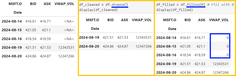
- Data Cleaning with Pandas: dropna(), fillna(), drop_duplicates(), astype()
- Transforming Data (creating new columns, applying function, grouping data)
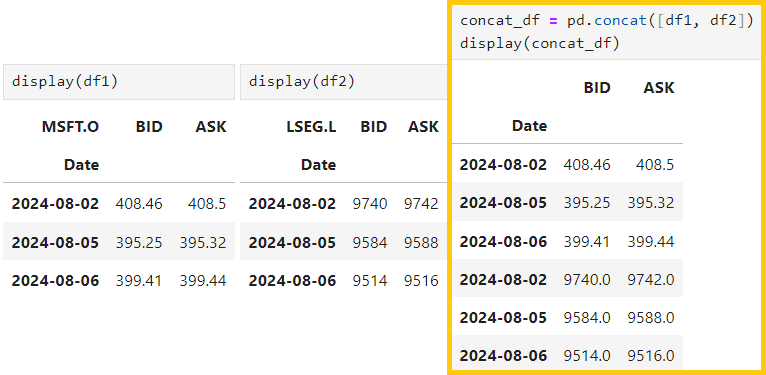
- Joining and Merging Dataframes: concat(), join(), merge()
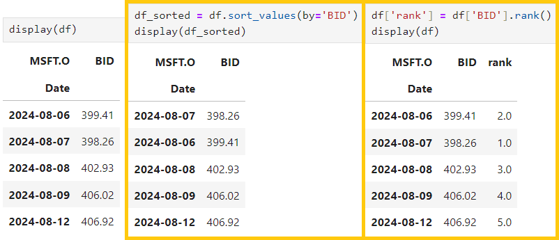
- Sorting and Ranking Data: sort_values(), rank()
- Advanced Dataframe Manipulations: pivot_table(), melt(), stack(), unstack()
Introduction to Pandas and Dataframes
Pandas, a very popular library in Python, helps us to work with data easily. You can think of it as a tool that allows us to play with data, like moving columns and rows in an Excel sheet. Pandas makes it easy to clean, modify, and analyze data, making it very useful in the data-related projects such as data science projects.
DataFrame is like a table with rows and columns. It's similar to a table in SQL or an Excel spreadsheet, making it easy to work with structured data and allow you to organize data in a way that is easy to read and work with.
Setting Up Your Environment
Here, I'm using Python version 3.12.4 with Python libraries: pandas version 2.2.2 and lseg.data version 2.0.0 to retrieve the data.
Pandas can be installed with the 'pip' command as below (Python and pip needed to be installed first). More detail of Pandas installation can be found in this page.
pip install pandas
Retrieving the data
Data can be loaded into the DataFrame from different sources, such as importing it from CSV/Excel files, JSON data, SQL Database or retriving the data from any Python libraries.
This is the code to import Pandas Python library into the current working Python file and read CSV file named 'file.csv' and assign it into df variable
import pandas as pd
df = pd.read_csv('file.csv')
In this article, we're retrieving the data from LSEG Data Library for Python, which provides a set of ease-of-use interfaces offering coders uniform access to the breadth and depth of financial data and services available on the LSEG Data Platform. The API is designed to provide consistent access through multiple access channels and target both Professional Developers and Financial Coders. Developers can choose to access content from the desktop, through their deployed streaming services, or directly to the cloud. With the LSEG Data Library, the same Python code can be used to retrieve data regardless of which access point you choose to connect to the platform.
The example code can be found in GitHub Example - Data Library Python, such as EX-1.01.01-GetData.ipynb. For example, let's retrieve data of MAMAA stocks (Meta, Amazon, Microsoft, Apple and Alphabet). To find the instruments and fields you're interested in, Data Item Browser can be used.
import lseg.data as ld
ld.open_session()
# Meta, Amazon, Microsoft, Apple and Alphabet
df = ld.get_data(
universe=['META.O', 'AMZN.O', 'MSFT.O', 'AAPL.O', 'GOOGL.O'],
fields=['TR.CommonName',
'TR.AlsoKnownAsName']
)
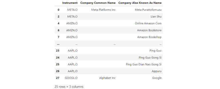
1) Basic Dataframe Operations
Basic operations that are commonly used to explore and understand data by viewing, selecting, and filtering data.
1.1 ) Viewing Data:
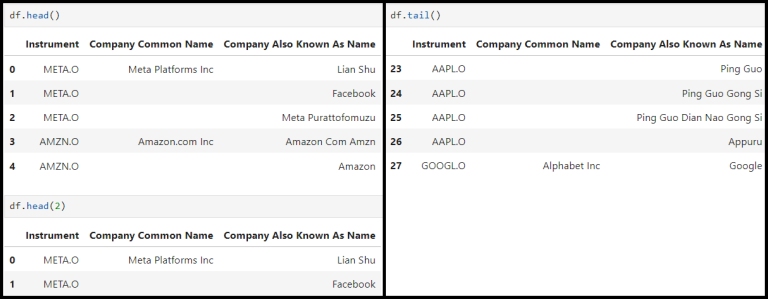
1.1.1 ) See the first few rows of a dataframe using 'head()' - default is 5 rows and you can put the number of rows of data you want to get as DataFrame.head(n)
- If n is negative value, the function returns all rows except the last |n| rows
- If n is larger than the number of rows, this function returns all rows
df.head()
1.1.2) Similar to head, to retrieve the last few rows of data, 'tail()' can be used
df.tail()
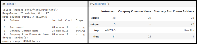
1.1.3) Getting summary of the data frame by using 'info()'
df.info()
1.1.4) See a summary of statistics with 'describe()'
df.describe()
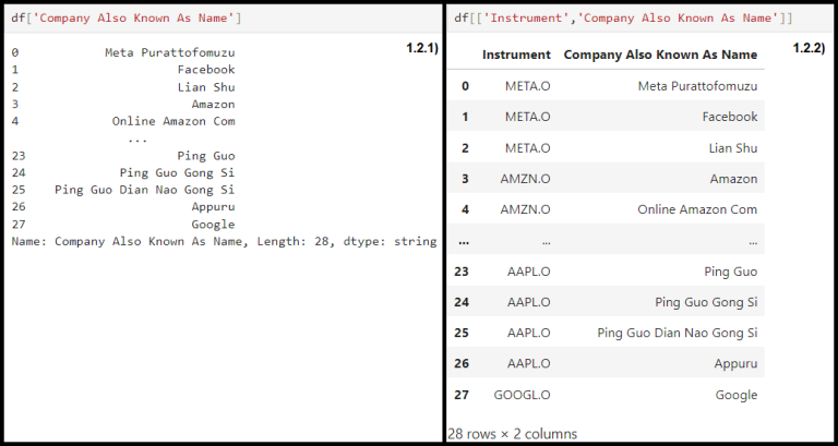
1.2) Selecting Data:
1.2.1 ) Select specific column
df['column_name']
1.2.2) Select multiple columns, use list of column as an input
df[['column1', 'column2']]
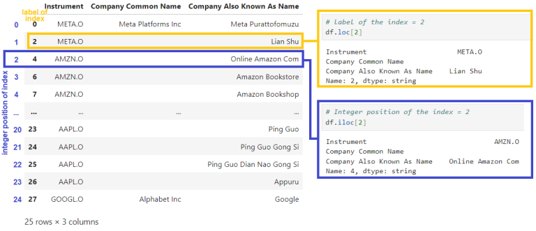
1.2.3) Select rows using 'loc[]' (label-based) and 'iloc[]' (integer-based) indexing
- Input of loc[] is a single label, e.g. 5 or 'a',
(5 is interpreted as a label of the index, and never as an integer position along the index)
df.loc[n]
- Input of iloc[] is an integer, e.g. 5
df.iloc[n]
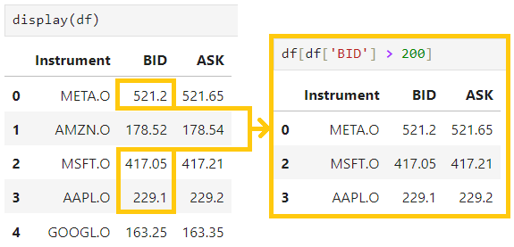
1.3) Filtering Data:
Rows can be filtered based on conditions, such as, to select the row that has value of the columm larger than n
df[df['column_name'] > n]
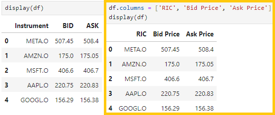
1.4) Changing Column Names:
Column names of a dataframe can be changed by assigning a new list of names to 'df.columns', or using the 'rename()' method to rename specific columns.
1.4.1 ) Renaming All Columns, replaces all column names with a new list of names, use the code below
df.columns = ['new_col1', 'new_col2', 'new_col3']
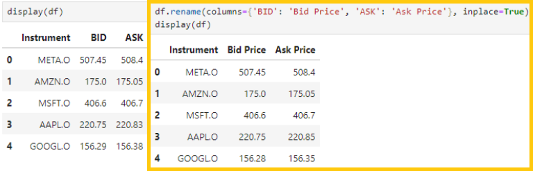
1.4.2) Renaming Specific Columns, if you only want to rename one or a few columns, use 'rename()'
Please note that 'inplace=True' updates the edited dataframe itself (the default value of this parameter is False, which will not update the original dataframe, but the dataframe with changes needs to be assigned to the new variable of dataframe)
df.rename(columns={'old_col1': 'new_col1', 'old_col2': 'new_col2'}, inplace=True)
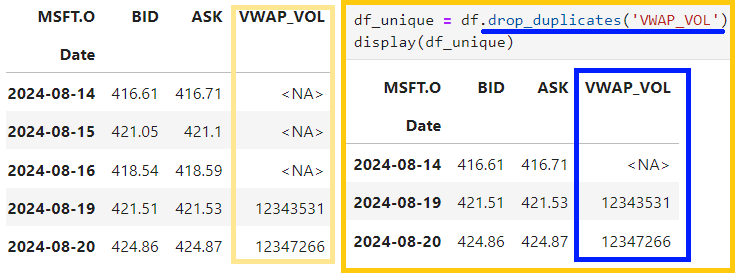
2.3) Removing duplicates by using 'drop_duplicates()' to remove duplicate rows
df_unique = df.drop_duplicates()
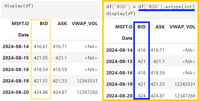
2.4) Changing data types of column using 'astype()'
df['column_name'] = df['column_name'].astype(int)
3) Transforming Data
Change data by creating new columns, applying function, and grouping data
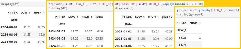
3.1 ) Adding new columns based on other columns
df['new_column'] = df['column1'] + df[column2']
3.2) Applying functions to a column using 'apply()'
df['plus 10'] = df['column1'].apply(lambda x: x+10)
3.3) Grouping data and perform calculations using 'groupby()'
grouped = df.groupby('column1').sum()
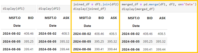
4.2) Joining dataframes with 'join()' for joining them on the index
df1.join(df2)
4.3) Merging dataframes based on a key column using 'merge()'
pd.merge(df1, df2, on='key_column')
6) Advanced Dataframe Manipulations
In this section, let's explore more complex dataframe manipulations that can help us reshape and aggregate data in different ways. These techniques are useful when we want to pivot data or change the layout of our dataframe for specific analyzes.
6.1 ) Creating pivot tables with 'pivot_table()'. This allows us to summarize data and group it in various ways with ease.
pivot = df.pivot_table(index='column1', columns='column2', values='column3', aggfunc='sum')
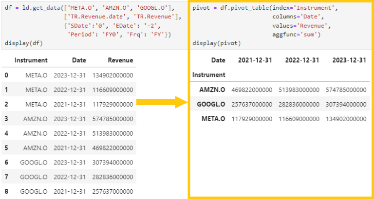
Imagine we have the dataframe that contains last 3 years of revenue data of these 3 companies and we want to find out the total revenue of each company. The pivot table can be created like this.
- Index='Instrument' specifies that the rows should be grouped by the 'Instrument' column
- columns='Date' creates separate columns for each 'Date'
- values='Revenue' indicates that the values in the table should be from 'Revenue' column
- aggfunc='sum' sums up the revenue for each combination of instrument and date. This can also be changed to other functions like 'mean', 'min', or 'max' based on what is needed.
df = ld.get_data(['META.O', 'AMZN.O', 'GOOGL.O'],
['TR.Revenue.date', 'TR.Revenue'],
{'SDate':'0', 'EDate': '-2',
'Period': 'FY0', 'Frq': 'FY'})
pivot = df.pivot_table(index='Instrument',
columns='Date',
values='Revenue',
aggfunc='sum')
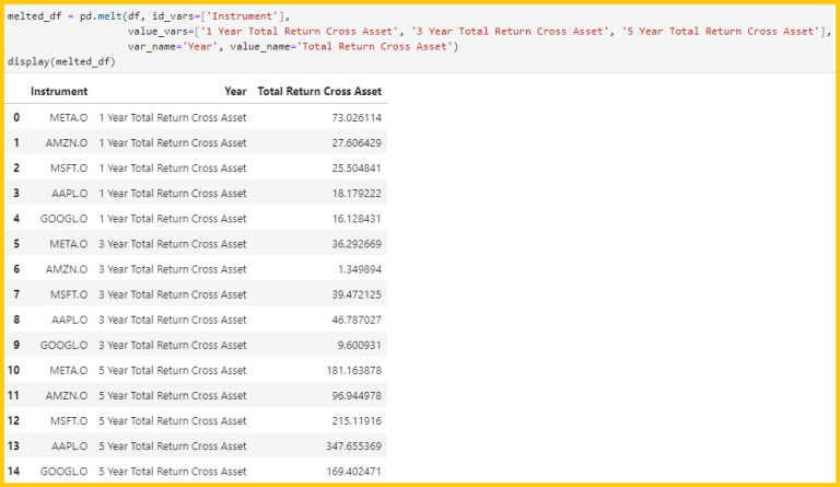
6.2) Reshaping data with 'melt()' to change the format. This is useful to tranform the data from wide format (many columns) to a long format (fewer columns, more rows). This is often required when we need to prepare the data for plotting or more advanced analysis.
melted_df = pd.melt(df, id_vars=['id_column'],
value_vars=['column1', 'column2'],
var_name='new_column_var', value_name='new_column_value')
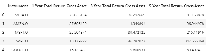
Let's say we have the dataframe which each column represents a total return cross asset on 1, 3, and 5 years period then we we're transforming it into a long format where each row represents total return cross asset for a specific instrument in a specific number of years period, as below.
- id_vars=['Instrument'], this column will remain unchanged, meaning the instrument RIC will stay the same for each row.
- value_vars=[''1 Year Total Return Cross Asset, ... , '5 Year Total Return Cross Asset'], are the columns that will be transformed into rows.
- var_name='Year' is the column name for the melted variable (inthis case, the year).
- value_name='Total Return Cross Asset', is the name of the new column where the values will be sorted.
df = ld.get_data(['META.O', 'AMZN.O', 'MSFT.O', 'AAPL.O', 'GOOGL.O'],
['TR.TotalReturn1YrCrossAsset', 'TR.TotalReturn3YrCrossAsset', 'TR.TotalReturn5YrCrossAsset'])
display(df)
melted_df = pd.melt(df, id_vars=['Instrument'],
value_vars=['1 Year Total Return Cross Asset', '3 Year Total Return Cross Asset', '5 Year Total Return Cross Asset'],
var_name='Year', value_name='Total Return Cross Asset')
display(melted_df)
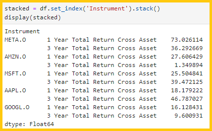
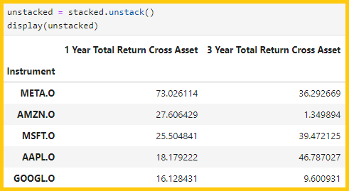
6.3) Reshaping data with 'stack()' and 'unstack()'
- stack() function is used to pivot the columns into rows
- unstack() function does the opposite, which pivots the rows into columns
df_stacked = df.stack()
df_unstacked = df_stacked.unstack()
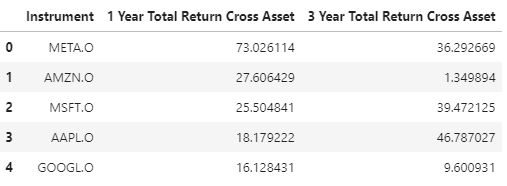
df = ld.get_data(['META.O', 'AMZN.O', 'MSFT.O', 'AAPL.O', 'GOOGL.O'],
['TR.TotalReturn1YrCrossAsset', 'TR.TotalReturn3YrCrossAsset'])
display(df)
stacked = df.set_index('Instrument').stack()
display(stacked)
unstacked = stacked.unstack()
display(unstacked)
Conclusion
In this beginners' guide to dataframe manipulation with Pandas, we've covered the essential functions that are the backbone of data analysis in Python from loading data and inspecting it, to filtering, grouping, and transforming. Pandas provides a powerful toolkit that simplifies working with complex datasets. By using practical examples and applying these techniques to datasets, you should now have a solid foundation to manipulate dataframes. Whether you're cleaning data, performing exploratory analysis, or preparing data for machine learning models, mastering these Pandas basics will signigicantly enhance your data science capabilities.
For further reading and more advanced tutorials, consider exploring the official Pandas documentation and using it with the datasets provided by LSEG via LSEG Data Library for Python.
- Register or Log in to applaud this article
- Let the author know how much this article helped you