

Last Updated: July 2025.
This article is outdated!! Please find an up-to-date article with the strartegic Data Library for Python on the Analysing S&P500 companies stocks with Beneish's M-Score and Altman's Z-Score article.
This article was written by the winner of 2021 Q.2 Refinitiv Academic Competition. It is aimed at Academics from Undergraduate level up.
Refinitiv Academic Article Competition
Refinitiv is pleased to host its Academic Article Competition.
This competition aims at helping students - from undergraduate to postdoctorate level - to publish their work on internationally recognized platforms and to aid them in (i) academic style writing, (ii) implementing code in their study, (iii) coding, (iv) financial knowledge, (v) developing a contacts network in the finance, and (vi) generating ideas for economics/finance papers.
It will have to be an economic or financial study, and in a style akin to these articles:
- Estimating Monthly GDP Figures Via an Income Approach and the Holt-Winters Model
- Investigating the effect of Company Announcements on their Share Price following COVID-19 (using the S&P 500)
- Information Demand and Stock Return Predictability (Coded in R)
- Computing Risk-Free Rates and Excess Returns from Zero-Coupon-Bonds
As per these examples, the length of the study in question is not a limit; there is no min. or max. length your article has to be to qualify. However, it needs to show and explain the code used in its study. It can be in any (reasonable) format (such as LaTeX, PDF, Word, Markdown, …) but it would preferably be a Jupyter Notebook (you may choose to use Refinitiv’s CodeBook to write it). You will also need to use Refintiv APIs/data-sets before being published on our Developer Portal – were it to win the competition.
There is no min. or max. number of winners; any work exceeding our standards will be selected for publication. Thus, do not hesitate to share this with your colleagues, informing them of this opportunity, they are not competitors, but collaborators; you may even choose to work together on this project.
We are ready and happy to provide any help in writing such articles. You can simply email Jonathan Legrand - the Competition Leader - at jonathan.legrand@refinitiv.com .
Abstract
This article aims to study the stock returns of companies that are likely to have manipulated their earnings and that are in a difficult financial situation (higher probability of bankruptcy). To that aim, the Beneish M-Score and the Altman Z-Score models are employed for the companies listed in the S&P500 using the data obtained from Refinitiv's Eikon API from 1995 to 2020.
Using the original cut-offs defined by the creators of the respective ratios, the results show that those companies that are more likely to have manipulated their earnings obtain an average of 207 basis points (BPS) less every year, while those that have a higher chance of bankruptcy obtain an average of 132 less BPS each year. However, when combining the two models the results obtained are an average of 862 BPS each.
In addition, by using the quintiles across each sector every year, the results obtained show that those companies in the fifth quintile of their sector’s m-score and in the first quintile of their sector’s z-score produce an average of 308 BPS less each year. Thus the z-score and the m-score can be useful for selecting better performing stocks.
1. Introduction
During the last few years, there has been an increase in the questioning of the usefulness of financial statements for investors. The publication of the book The End of Accounting (2016) supported the existence of a downtrend in the usefulness of financial statements. Although other authors have supported the need for improvement in terms of reporting standards (Papa, 2018), they still defend a less extreme position or even support the growing utility of reporting ESG factors as a possible solution (Dreyer CFA, 2020). The flexibility of accounting standards is a double edge sword that gives managers a better position for manipulating earnings through different accounting choices.
In this article, the usefulness of financial analysis is analyzed by screening the stocks using the z-score and the m-score and studying the stock prices. Those companies with low probability of having manipulated earnings and low probability of bankruptcy are considered for a long position whereas those with high probabilities are considered for a short position.
2. Literature Review
Beneish M-Score
The Beneish m-score model (Beneish et al., 1999) is a quantitative model of eight variables obtained from financial statements that estimates the probability of earnings management for a given financial statement. The eight variables and the m-score are defined as
$$\text{Days Sales in Receivables Index (DSRI)} = \frac{\frac{Receivables_t}{Sales_t}}{\frac{Receivables_{t-1}}{Sales_{t-1}}} .$$
To calculate the DSRI we define the following function
def DSRI(df):
return (df["receivables"] / df["sales"]) / (df["receivables_t2"] / df["sales_t2"])
$$\text{Gross Margin Index (GMI) } = \frac{\text{Gross margin}_{t-1}}{\text{Gross margin}_t} $$
To calculate the GMI we define the following function
def GMI(df):
return (df["sales_t2"] - df["cogs_t2"]) / (df["sales"] - df["cogs"])
$$\text{Asset Quality Index (AQI) } = \frac{1 - \frac{\text{Property plant and equipment}_t + \text{ Current assets}_t}{\text{Total assets}_t}}{1-\frac{\text{Property plant and equipment}_{t-1} + \text{ Current assets}_{t-1}}{\text{Total assets}_{t-1}}}$$
To calculate the AQI we define the following function
def AQI(df):
AQI_t1 = (1 - (df["ppe"] + df["current_assets"]) / df["total_assets"])
AQI_t2 = (1 - (df["ppe_t2"] + df["current_assets_t2"]) / df["total_assets_t2"])
return AQI_t1 / AQI_t2
$$\text{Sales Growth Index (SGI) } = \frac{Sales_t}{Sales_{t-1}}$$
To calculate the SGI we define the following function
def SGI(df):
return (df["sales"] / df["sales_t2"])
$$\text{Depreciation Index (DEPI) } = \frac{\frac{Depreciation_{t-1} + \text{ Property plant and equipment}_{t-1}}{Depreciation_{t-1}}}{\frac{Depreciation_t + \text{ Property plant and equipment}_t}{Depreciation_t}}$$
To calculate the DEPI we define the following function
def DEPI(df):
DEPI_t1 = (df["depreciation"] / (df["depreciation"] + df["ppe"]))
DEPI_t2 = (df["depreciation_t2"] / (df["depreciation_t2"] + df["ppe_t2"]))
return DEPI_t1 / DEPI_t2
$$\text{Sales General and Administrative Expenses Index (SGAI) } = \frac{\frac{\text{Sales, general, and administrative expenses}_t}{Sales_t}}{\frac{\text{Sales, general, and administrative expenses}_{t-1}}{Sales_{t-1}}}$$
To calculate the SGAI we define the following function
def SGAI(df):
return (df["sga"] / df["sales"]) / (df["sga_t2"] / df["sales_t2"])
$$\text{Leverage Index (LVGI) } = \frac{Leverage_t}{Leverage_{t-1}}$$
To calculate the LVGI we define the following function
def LVGI(df):
return (df["debt"] / df["total_assets"]) / (df["debt_t2"] / df["total_assets_t2"])
$$\text{Total Accruals to Total Assets (TATA) } = \frac{\text{Inc. before extr. items} - \text{ Cash from operations}}{\text{Total assets}}$$
To calculate the TATA we define the following function
def TATA(df):
return (df["inc"] - df["ncf"]) / df["total_assets"]
$$ \text{M-Score} = –4.84 + 0.920 (DSRI) + 0.528 (GMI) + 0.404 (AQI) + 0.892 (SGI) + 0.115 (DEPI) -0.172 (SGAI) + 4.679 (TATA) – 0.327 (LVGI) $$
The companies whose m-score are higher than -1.78 are considered likely to have manipulated their earnings, while those under -2.22 are considered that have fairer reports. To calculate the M-Score we define the following function
def get_m_score(df):
df["m-score"] = -4.84 + 0.92 * DSRI(df) + \
0.528 * GMI(df) + \
0.404 * AQI(df) + \
0.892 * SGI(df) + \
0.115 * DEPI(df) + \
-0.172 * SGAI(df) + \
4.679 * TATA(df) + \
-0.327 * LVGI(df)
There is sounding literature studying the Beneish m-score model for analyzing manipulations of earnings of companies. This model proved effective for Polish listed companies, excluding the financial sector, since 2010 (Hołda, 2020), for companies in Turkey from 2005 to 2017 (Özcan, 2018), for companies sanctioned and fined by the Financial Services Authority between 2012 and 2016 (Alfian and Triani, n.d.) and for Malaysian companies from 1996 to 2014 (Kamal, Salleh and Ahmad, 2016).
Furthermore, years after its publication, the Beneish m-model still classifies multiple stocks listed on different markets as likely to have manipulated earnings. Manufacturing and trading companies listed on the Ghana Stock Exchange from 2008 to 2017 were very likely to engage in earnings management (Anning and Adusei, 2020). In addition, the z-score showed good results in predicting the manipulation of financial statements. Furthermore, for companies listed on the Ghana Stock Exchange from 2011 to 2016 it was found that big companies as well as small companies engaged in earnings management (Adu-Gyamfi, 2020). 55 % of the companies listed on the Bucharest Stock Exchange from 1998 to 2017 were likely to have managed their earnings based on the m-score, and reviewing the m-score for companies across other countries it is concluded that 67% of the companies reviewed have manipulated at least half of their financial statements (Mihalcea, 2020). In addition, that paper showed that on average those companies which are likely to have manipulated their earnings exhibited better results for their reported ratios.
Altman Z-Score
The Altman z-score model (Altman, 1968) is a quantitative model of five variables for predicting the probability of bankruptcy of a company. The z-score is defined as follows:
$$\begin{array} \text{Z-Score } &= 1.2 \left( \frac{\text{Net working capital}}{\text{Total assets}} \right) + 1.4 \left( \frac{\text{Retained earnings}}{\text{Total assets}} \right) + 3.3 \left(\frac{\text{EBIT}}{\text{Total assets}}\right) \\ & + 0.6 \left(\frac{\text{Market value of equity}}{\text{Book value of liabilities}}\right) + 1.0 \left(\frac{\text{Sales}}{\text{Total assets}}\right) \end{array} $$
Companies with a Z-score over 3 are considered having a low risk of bankruptcy while those under 1.81 have a higher risk. To calculate the M-Score we define the following function
def get_z_score(df):
df["z-score"] = 1.2 * df['working_capital_to_assets'] + \
1.4 * df['retained_to_assets'] + \
3.3 * df['ebit_to_assets'] + \
0.6 * df['market_cap_to_liabilities'] + \
1.0 * df['asset_turnover']
For companies listed in the Kuwaiti Stock Market, excluding banking and insurance companies, the combination of the m-score along with the z-score resulted in higher precision of classifying financial frauds (Akra and Chaya, 2020). For companies on selected sectors in Iran both models proved effective from 2009 to 2016 (Taherinia and Talebi, n.d.).
Although still supporting the effectiveness of the z-score and the m-score, for auditor’s fraud detection gap on the Gulf Cooperation Council companies from 2015 to 2017, the Dechow F-score was superior for detecting fraud (Hakami et al., 2020).
3. Model definition, data and analysis
The companies analyzed are the constituents of the S&P 500 at the start of each year since 1995 to the end of 2020. For each year, the m-score and the z-score are calculated using the latest financial statements.
The companies whose m-score is higher than -1.78 and a z-score lower than 1.81 are companies likely to have manipulated their earnings and which also have a higher probability of bankruptcy. On the opposite side, companies whose m-score is lower than -2.22 and z-score is higher than 3 are considered companies with fairer earnings reports and low probability of bankruptcy.
Assumptions
• The companies with missing data for calculations are ignored.
• The returns of each company are those obtained during the following fiscal year, hence for some companies there is a lag depending on the date of publication of their latest financial statements and the stock price might have already reflected these financial statements.
• For certain companies, whose reporting dates are during the start of the year following their fiscal year-end, the results include the period during which the financial statement was not available yet.
Getting to the Coding
To start with we need to make some imports
import sys
print(sys.version) # 3.7.9 (default, Aug 31 2020, 17:10:11) [MSC v.1916 64 bit (AMD64)]
3.7.9 (default, Aug 31 2020, 17:10:11) [MSC v.1916 64 bit (AMD64)]
import eikon as ek # 1.1.18
import pandas as pd # 1.1.5
import numpy as np # 1.18.5
import plotly.express as px
import plotly.graph_objects as go
import plotly as pyo # 4.13.0
# for i,j in zip(["eikon", "pandas", "numpy", "plotly"],[ek, pd, np, pyo]):
# print("The " + i + " Python library used here is version " + j.__version__)
The versions of the different libraries are showed to facilitate reproductions
We will set the key for the API, this key is obtained using the Eikon APP to generate keys
# The key is placed in a text file so that it may be used in this code without showing it itself:
eikon_key = open("eikon.txt","r")
ek.set_app_key(str(eikon_key.read()))
# It is best to close the files we opened in order to make sure that we don't stop any other services/programs from accessing them if they need to:
eikon_key.close()
We define the elements we want to analyze
chain = '0#.SPX' # Constituents of the SPX
We define the dates for our study, as we need data from financial statements reported during the previous two years our first date is 1993, and our last date is 2021 because we need the returns up to the last date
dates = pd.date_range('1993', '2020', freq = 'YS')
We define the fields needed for our study
fields = [
'TR.TotalReturn52Wk', # 52 Week Returns
"TR.GICSSector" # GICS Sector
]
beneish_fields = [
"TR.F.LoansRcvblTot", # Receivables
"TR.F.TotRevBizActiv", # Sales
"TR.F.COGSTot", # Costs of goods sold
"TR.F.PPEGrossTot", # Property plant and equipment
"TR.F.TotCurrAssets", # Current assets
"TR.F.TotAssets", # Total assets
"TR.F.DeprTot", # Depreciation
"TR.F.SGATot", # Sales General and Administrative Expenses
"TR.F.IncBefDiscOpsExordItems", # Income before discontinued operations and extraordinary items
"TR.F.NetCashFlowOp", # Net cash flow from operating activities
"TR.F.DebtTot" # Total debt
]
altman_fields = [
"TR.F.WkgCaptoTotAssets", # Working capital to total assets
"TR.F.RetainedEarntoTotAssets", # Retained earnings to total assets
"TR.F.EBITToTotAssets", # EBIT to total assets
"TR.F.MktCapToTotLiab", # Market value of equity to liabilities
"TR.F.AssetTurnover" # Asset turnover
]
model_fields = beneish_fields + altman_fields
We want to create two dictionaries to store the limit values of the first and the fifth quantile for the z-score and for the m-score
score_columns = ["z-score", "m-score"]
long_quantiles = {date:{column:{} for column in score_columns} for date in dates}
short_quantiles = {date:{column:{} for column in score_columns} for date in dates}
We want to create two dictionaries to rename the columns of the dataframe that we will create, the second dictionary called columns_t2 appends "_t2" at the end of each column to distinguish them from the other columns
columns = {
'Loans & Receivables - Total': "receivables",
'Revenue from Business Activities - Total': "sales",
'Cost of Revenues - Total': "cogs",
'Property Plant & Equipment - Gross - Total': "ppe",
'Total Current Assets': 'current_assets',
'Total Assets': "total_assets",
'Depreciation - Total': "depreciation",
'Selling General & Administrative Expenses - Total': 'sga',
'Income before Discontinued Operations & Extraordinary Items': 'inc',
'Net Cash Flow from Operating Activities': 'ncf',
'Debt - Total': 'debt',
'Working Capital to Total Assets': 'working_capital_to_assets',
'Retained Earnings - Total to Total Assets': 'retained_to_assets',
'Earnings before Interest & Taxes (EBIT) to Total Assets': 'ebit_to_assets',
'Market Capitalization to Total Liabilities': 'market_cap_to_liabilities',
'Asset Turnover': 'asset_turnover'
}
columns_t2 = {x: f"{y}_t2" for x, y in columns.items()}
We create an empty dataframe to store all the results in a single dataframe
full_df = pd.DataFrame()
We are iterating over each year from 1995 to 2020, we create the parameters to get the financial statements two years ago, then one year ago and then to obtain the following year return for the companies constituents of the S&P500 at the start of that year.
We create dataframes with data obtained from eikon and we store only the results and ignore the errors, after that, we drop the missing values, rename the columns and set the index to the instruments. We join the dataframes and we store only the instruments where all parameters are available. Then, we store that year as a column and compute the z-score and the m-score for the joined dataframe and drop the strange values.
Finally, we store the values of the quintiles in our dictionaries for each sector and for each year. In addition, we store that year results in our previously created dataframe and we print the date to view the progress of our loop.
# This step takes some minutes to complete, if the connection is lost in between it is possible to change the dates variable
# Setting the starting date in the dates variables to the year before the last year printed allows it to continue
# However, the starting date in the dates variable should be changed again to 1993 for later use
for i, date in enumerate(dates[2:-1],2):
# Dates conversion to obtain the data from eikon
date_0 = date.to_period('D')
date_1 = dates[i-1].to_period('D')
date_2 = dates[i-2].to_period('D')
date_end = dates[i+1].to_period('D')
# Creation of parameters to get data for selected years from eikon
parameters_t2 = {'SDate': f"{date_2}", 'EDate': f"{date_1}", 'FRQ': 'FY'}
parameters_t1 = {'SDate': f"{date_1}", 'EDate': f"{date_0}", 'FRQ': 'FY'}
parameters_last = {'SDate': f"{date_end}"}
# Here we obtain the data and store it in dataframes, get_data returns a tuple containing (dataframe, errores)
# we are only interested in the dataframe so we ignore the errors
df_t2 = ek.get_data(f"{chain}({date_0})", model_fields, parameters_t2)[0]
df_t1 = ek.get_data(f"{chain}({date_0})", model_fields, parameters_t1)[0]
rets = ek.get_data(f"{chain}({date_0})", fields, parameters_last)[0]
# We drop the instruments with missing rows, rename the columns and set the index to that instrument
df_t1 = df_t1.dropna().rename(columns = columns).set_index('Instrument')
df_t2 = df_t2.dropna().rename(columns = columns_t2).set_index('Instrument')
rets = rets.dropna().rename(columns = {
'52 Week Total Return': 'returns',
'GICS Sector Name': 'sector'
}).set_index('Instrument')
# We join the dataframes and store the year as a column
df = rets.join(df_t1, how = "inner").join(df_t2, how = "inner")
df["date"] = date.to_period('Y')
# We compute the z-score, the m-score and drop the strange values
get_z_score(df)
get_m_score(df)
df = df.replace([np.inf, -np.inf, ""], np.nan).dropna()
# We fill our dictionaries with the data of the first and the fifth quintile
for column in score_columns:
for sector in df["sector"].unique():
long_quantiles[date][column][sector] = df[df["sector"] == sector][column].quantile(0.8)
short_quantiles[date][column][sector] = df[df["sector"] == sector][column].quantile(0.2)
# Finally we store the data in our previously created dataframe and print the date to view the progress
full_df = full_df.append(df, ignore_index = True)
print(date)
1995-01-01 00:00:00
1996-01-01 00:00:00
1997-01-01 00:00:00
1998-01-01 00:00:00
1999-01-01 00:00:00
2000-01-01 00:00:00
2001-01-01 00:00:00
2002-01-01 00:00:00
2003-01-01 00:00:00
2004-01-01 00:00:00
2005-01-01 00:00:00
2006-01-01 00:00:00
2007-01-01 00:00:00
2008-01-01 00:00:00
2009-01-01 00:00:00
2010-01-01 00:00:00
2011-01-01 00:00:00
2012-01-01 00:00:00
2013-01-01 00:00:00
2014-01-01 00:00:00
2015-01-01 00:00:00
2016-01-01 00:00:00
2017-01-01 00:00:00
2018-01-01 00:00:00
2019-01-01 00:00:00
We already have all the data required for our study so now we are going to plot it to observe the distribution for the m-score and the z-score across sectors or dates using plotly.express
First, we create a function to plot the selected score across sectors, for visualization purposes we will limit the values of the m-score between -5 and 0 and the z-score between -10 and 15
# We define the auxiliary functions to limit the extreme values
def to_z_range(num):
upper = 15
lower = -10
if num > upper: return upper
elif num < lower: return lower
else: return num
def to_m_range(num):
upper = 0
lower = -5
if num > upper: return upper
elif num < lower: return lower
else: return num
# We define a function with two parameters to plot the m-score or the z-score and across sectors or dates
def plot_score(m_score = True, sectors = True, title = ""):
# We create some variables to make the neccesary changes depending on the selected parameters
col = "m-score" if m_score else "z-score"
fun = to_m_range if m_score else to_z_range
title = "M-Score" if m_score else "Z-Score"
across = "sector" if sectors else "date"
height = 1000 if sectors else 1500
# We define a boxplot, set the colors to the sector and plot the m-score in the y-axis
fig = px.box(
color = full_df[across] if sectors else None,
y = None if sectors else full_df[across].astype(str),
x = full_df[col].apply(fun),
template = "plotly_white",
orientation = 'h',
width = 1000,
height= height
)
# We style the titles and fonts for our plot
fig.update_layout(
title = title,
xaxis_title = title,
yaxis_title = across.capitalize(),
legend_title = across.capitalize(),
legend_traceorder = "reversed",
font = dict(size = 18),
)
# We dont want to plot all the extreme values as only one point
fig.update_traces(jitter = 1)
# Finally we show the plot
fig.show()
First we will plot the m-score across the different sectors
plot_score(m_score = True, sectors = True, title = "M-Score across sectors")
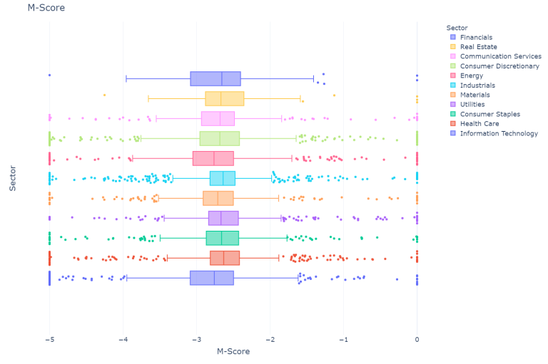
The m-score across sectors stays relatively centered around -2.75 however there are more extreme values as the highest m-score in the data is 967 and the lowest value is -1762 as can be seen below
print("The highest m-score value is :", full_df["m-score"].max())
print("The lowest m-score value is :", full_df["m-score"].min())
The highest m-score value is : 967.5524667180356
The lowest m-score value is : -1762.6651000656682
The m-score can be further explored and we could compute other statistics, nevertheless now we are going to plot the z-score across sectors
plot_score(m_score = False, sectors = True, "Z-Score across sectors")
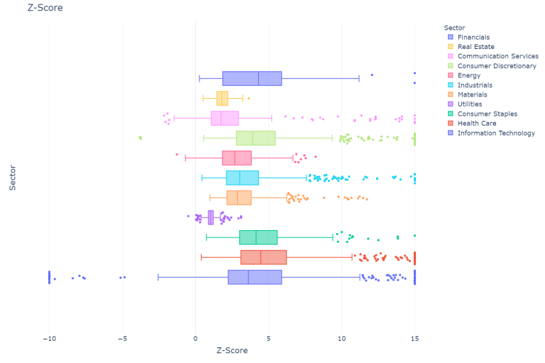
For the z-score the results are more varied, especially for the IT sector which has the most negative outliers. In addition, the median value of the z-score is more distributed across the sectors, particularly the utilities, the communication services and the real estate sectors exhibit a lower value, although in the original paper (Altman 1968), Altman justified lower values for the real state and the manufacturing sectors.
Now we are going to plot the m-score and the z-score across the dates to get an idea of the historical change
plot_score(m_score = True, sectors = False, "M-Score across years")
plot_score(m_score = False, sectors = False, "Z-Score across years")
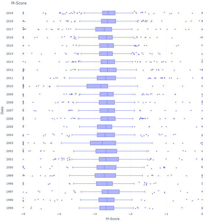
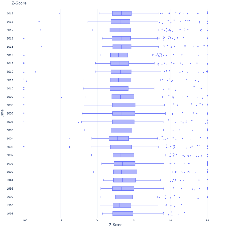
The median of both scores stays relatively stable over the years considered. The values are calculated below:
print("The mean m-score value is :", full_df["m-score"].median())
print("The mean z-score value is :", full_df["z-score"].median())
The mean m-score value is : -2.67
The mean z-score value is : 3.15
Now we are going to create the screening filters. We create a filter for companies having an m-score lower than -2.22 and a z-score higher than 3. Then, we create another filter for m-scores higher than -1.78 and z-scores lower than 1.81.
long_z_score = (full_df["z-score"] > 3)
short_z_score = (full_df["z-score"] < 1.81)
long_m_score = (full_df["m-score"] < -2.22 )
short_m_score = (full_df["m-score"] > -1.78 )
long_screening = long_z_score & long_m_score
short_screening = short_z_score & short_m_score
We are ready to test the results of our models, first we will create two empty lists to store our results. For each year, we store the a tuple consisting of the year, the number of stocks after applying the screening filters and the average returns of the companies that fulfilled the criteria. Finally, we convert the lists to arrays and we create two dataframes to facilitate the analysis. To facilitate further analysis we define a function that accepts the screening filters as parameters.
def get_df_results(long_filter, short_filter):
long_results = []
short_results = []
for date in full_df["date"].unique():
date = str(date)
long_universe = long_filter & (full_df["date"] == date)
short_universe = short_filter & (full_df["date"] == date)
long_results.append((
date,
len(full_df[long_universe]),
full_df["returns"][long_universe].astype(np.float64).mean()
))
short_results.append((
date,
len(full_df[short_universe]),
full_df["returns"][short_universe].astype(np.float64).mean()
))
long_results = np.array(long_results)
short_results = np.array(short_results)
df_long = pd.DataFrame(long_results[:, 1:], long_results[:, 0], ["stocks", "returns"], np.float64)
df_short = pd.DataFrame(short_results[:, 1:], short_results[:, 0], ["stocks", "returns"], np.float64)
return df_long, df_short
Now we will create 6 dataframes, one based on the m-score screening alone, one based on the z-score alone and one combining both screening methods.
df_m_long, df_m_short = get_df_results(long_m_score, short_m_score)
df_z_long, df_z_short = get_df_results(long_z_score, short_z_score)
df_long, df_short = get_df_results(long_screening, short_screening)
To facilitate visualization we join the long and short dataframes and compute the returns of the companies in the long screening minus the returns of those in the short screening
def join_df(df_l, df_s):
df_j = df_l.join(df_s, how = "inner", lsuffix = "_long", rsuffix = "_short")
df_j["results"] = df_j["returns_long"] - df_j["returns_short"]
return df_j
df_m_joined = join_df(df_m_long, df_m_short)
df_z_joined = join_df(df_z_long, df_z_short)
df_joined = join_df(df_long, df_short)
Now we are going to define a function to plot the results across the years, we want to visualize the returns of the stocks that passed the long criteria, the short criteria and the difference between them.
def plot_returns(df, title = ""):
fig = go.Figure()
fig.add_trace(go.Scatter(x = df.index,
y = df["returns_long"],
mode ='lines+markers',
name ='long screening'))
fig.add_trace(go.Scatter(x = df.index,
y = df["returns_short"],
mode ='lines+markers',
name ='short screening'))
fig.add_trace(go.Scatter(x = df.index,
y = df["results"],
mode ='lines+markers',
name ='results'))
fig.update_layout(
title = title,
xaxis_title = "Dates",
yaxis_title = "Returns",
template = "plotly_white",
font = dict(size = 18),
height = 800,
width = 1000)
fig.show()
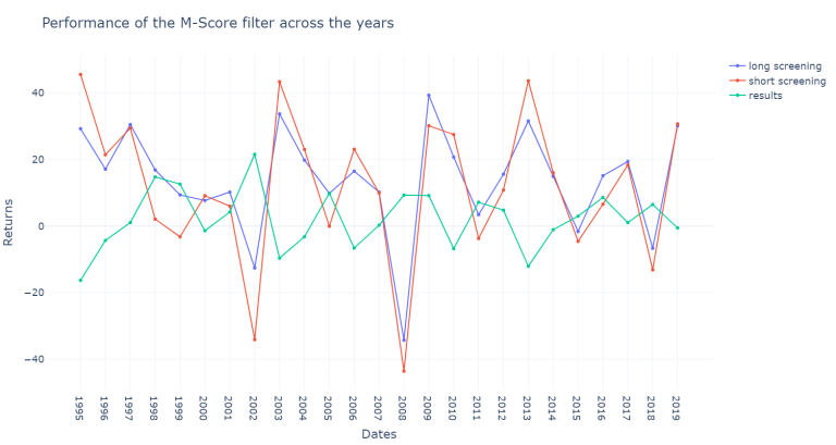
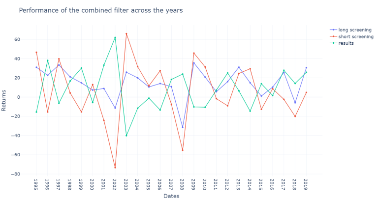
Before plotting the results we will compute the average performance of our screening method. As we can see below the filters alone perform better than the joined filter which produces worse returns.
print("The m-score filter alone produces a yearly average of :", round(100*df_m_joined["results"].mean()), "BPS")
print("The z-score filter alone produces a yearly average of :", round(100*df_z_joined["results"].mean()), "BPS")
print("The joined filter produces a yearly average of :", round(100*df_joined["results"].mean()), "BPS")
The m-score filter alone produces a yearly average of : 207 BPS
The z-score filter alone produces a yearly average of : 132 BPS
The joined filter produces a yearly average of : 862 BPS
However, when we compute the average of companies in our filter it seems that very few companies passed the joined criteria for the short side. On average only 4.32 companies passed the combined short criteria
print(df_m_joined["stocks_long"].mean(), "companies passed the m-score long criteria and",
df_m_joined["stocks_short"].mean(), "companies passed the short")
print(df_z_joined["stocks_long"].mean(), "companies passed the z-score long criteria and",
df_z_joined["stocks_short"].mean(), "companies passed the short")
print(df_joined["stocks_long"].mean(), "companies passed the combined long criteria and",
df_joined["stocks_short"].mean(), "companies passed the short")
192.68 companies passed the m-score long criteria and 14.08 companies passed the short
118.08 companies passed the z-score long criteria and 49.72 companies passed the short
102.6 companies passed the combined long criteria and 4.32 companies passed the short
As we can see below, the results across the years are quite volatile for the m-score, however since 2005 the results become more stable and the companies in the long screening outperform the companies in the short screening in a more consistent way.
plot_returns(df_m_joined, "Performance of the M-Score filter across the years")
The results for the z-score are also volatile across the years.
plot_returns(df_z_joined, "Performance of the Z-Score filter across the years")

By observing the results of the combined screening method we can notice how 1998 was the worst performing year by far
plot_returns(df_joined, "Performance of the combined filter across the years")
To test the results of the m-score and the z-score on a more balanced universe of stocks, now we are going to create the screening methods using our previously computed quintiles instead of the fixed values for the m-score and the z-score. In addition, we will separate the results across sectors. First we define a variable to store the sectors.
sectors = full_df["sector"].unique()
Now we are going to compare the results across sectors and instead of screening the stocks using fixed numbers for the z-score and the m-score we use the quintiles across sectors that we stored in dictionaries before. We start with a few modifications to create two dataframes to store the results for each year and each sector using our new screening method. Finally, we join the two dataframes using our previously defined function
def get_df_modified(z_score = True, m_score = True):
long_results = []
short_results = []
for date in dates[2:]:
for sector in sectors:
# If there is missing data for a sector on a given year we skip it
if z_score:
if (sector not in long_quantiles[date]["z-score"].keys() or
sector not in short_quantiles[date]["z-score"].keys()): continue
if m_score:
if (sector not in long_quantiles[date]["m-score"].keys() or
sector not in short_quantiles[date]["m-score"].keys()): continue
long_universe = ((full_df["date"] == str(date)) &
(full_df["sector"] == sector))
short_universe = ((full_df["date"] == str(date)) &
(full_df["sector"] == sector))
if z_score:
long_universe = (long_universe &
(full_df["z-score"] >= long_quantiles[date]["z-score"][sector]))
short_universe = (short_universe &
(full_df["z-score"] <= short_quantiles[date]["z-score"][sector]))
if m_score:
long_universe = (long_universe &
(full_df["m-score"] <= long_quantiles[date]["m-score"][sector]))
short_universe = (short_universe &
(full_df["m-score"] >= short_quantiles[date]["m-score"][sector]))
long_results.append((
date,
sector,
len(full_df[long_universe]),
full_df["returns"][long_universe].astype(np.float64).mean()
))
short_results.append((
date,
sector,
len(full_df[short_universe]),
full_df["returns"][short_universe].astype(np.float64).mean()
))
long_results = np.array(long_results)
short_results = np.array(short_results)
cols = ["stocks", "returns"]
# We want to create a multiindex Dataframe containing the year and the sector, thus we first create the multiindex
long_arrays = [long_results[:, 0], long_results[:, 1]]
short_arrays = [short_results[:, 0], short_results[:, 1]]
long_index = pd.MultiIndex.from_arrays(long_arrays, names=["date", "sector"])
short_index = pd.MultiIndex.from_arrays(short_arrays, names=["date", "sector"])
# Now we create the multiindex Dataframes
df_long_sectors = pd.DataFrame(long_results[:, 2:], long_index, cols, np.float64)
df_short_sectors = pd.DataFrame(short_results[:, 2:], short_index, cols, np.float64)
# Finally, we return the joined Dataframe
return join_df(df_long_sectors, df_short_sectors)
We define three dataframes, one for z-score, one for m-score filters alone and one for both filters combined
df_m_only = get_df_modified(z_score = False, m_score = True)
df_z_only = get_df_modified(z_score = True, m_score = False)
df_mix_only = get_df_modified(z_score = True, m_score = True)
Now we are going to plot the results across sectors and across years.
def plot_new_models(df_joined_sectors, title):
fig = go.Figure()
for sector in sectors:
fig.add_trace(go.Scatter(x=df_joined_sectors.xs(sector, level="sector").index,
y=df_joined_sectors.xs(sector, level="sector")["results"],
mode = 'lines+markers',
name = sector))
fig.update_layout(
title = title,
xaxis_title = "Dates",
yaxis_title = "Returns",
template = "plotly_white",
font = dict(size = 18),
height = 800,
width = 1000)
fig.show()
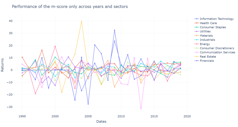
plot_new_models(df_m_only, "Performance of the m-score only across years and sectors")
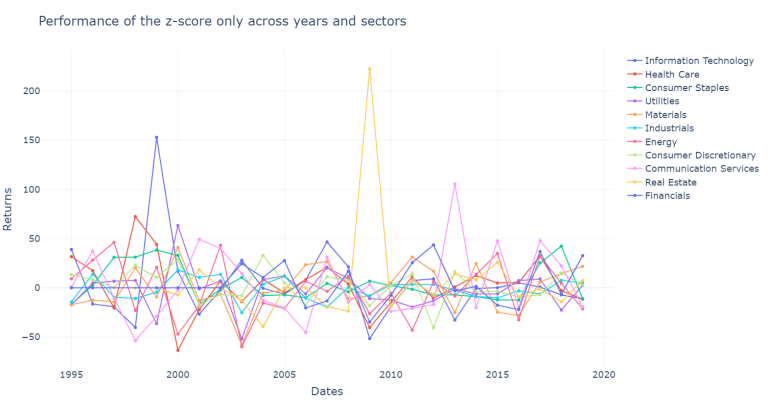
plot_new_models(df_z_only, "Performance of the z-score only across years and sectors")
plot_new_models(df_mix_only, "Performance of the combined screening method across years and sectors")
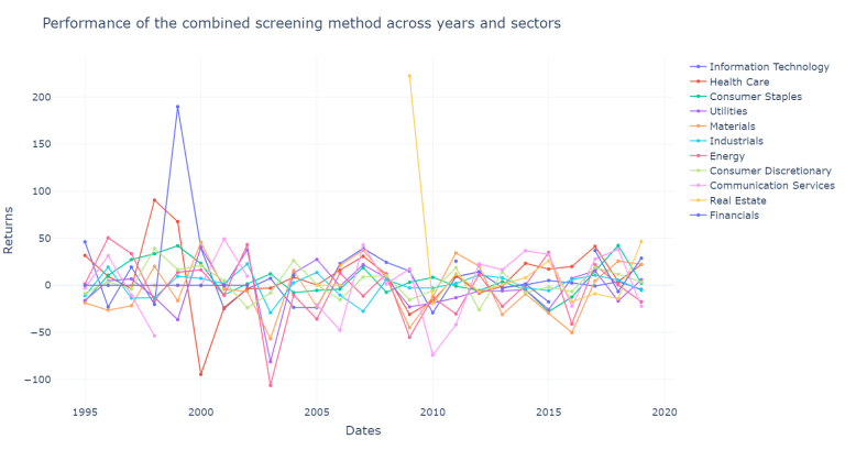
There is a lot of information that we can analyze, so it is bettet to summarize it, we are first going to compute the results across sectors and store the results.
sectors_m_score_results = []
sectors_z_score_results = []
sectors_mix_score_results = []
for sector in sectors:
sectors_m_score_results.append(df_m_only.xs(sector, level = "sector")["results"].mean())
sectors_z_score_results.append(df_z_only.xs(sector, level = "sector")["results"].mean())
sectors_mix_score_results.append(df_mix_only.xs(sector, level = "sector")["results"].mean())
Now we are going to do the same but across the years.
dates_m_score_results = []
dates_z_score_results = []
dates_mix_score_results = []
for date in df_mix_only.xs(slice(None), level = "sector").index.unique():
dates_m_score_results.append(df_m_only.xs(date, level = "date")["results"].mean())
dates_z_score_results.append(df_z_only.xs(date, level = "date")["results"].mean())
dates_mix_score_results.append(df_mix_only.xs(date, level = "date")["results"].mean())
Let's now plot the results first across sectors and then across years for better visualization.
def plot_results_across(df, across_dates = None, across_sectors = None, on = ""):
across_x = sectors if across_sectors else df.xs(slice(None), level = "sector").index.unique()
across_y = across_sectors if across_sectors else across_dates
subtitle = "Sectors" if across_sectors else "Dates"
title = f"Performance across {subtitle} for the {on} using quintiles"
fig = px.bar(x = across_x, y = across_y)
fig.update_layout(
title = title,
xaxis_title = subtitle,
yaxis_title = "Returns",
template = "plotly_white",
font = dict(size = 18),
height = 800,
width = 1000)
fig.show()
plot_results_across(df_m_only, across_dates = dates_m_score_results, on = "m-score")
plot_results_across(df_m_only, across_sectors = sectors_m_score_results, on = "m-score")
plot_results_across(df_z_only, across_dates = dates_z_score_results, on = "z-score")
plot_results_across(df_z_only, across_sectors = sectors_z_score_results, on = "z-score")
plot_results_across(df_mix_only, across_dates = dates_mix_score_results, on = "combined filter")
plot_results_across(df_mix_only, across_sectors = sectors_mix_score_results, on = "combined filter")
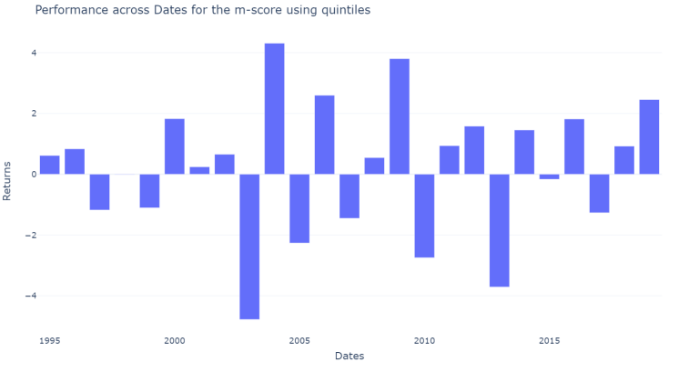
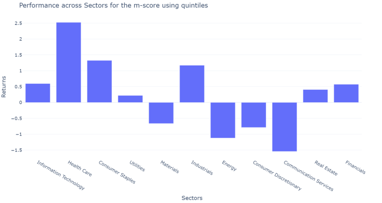
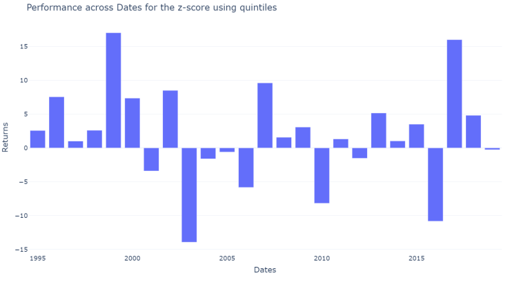
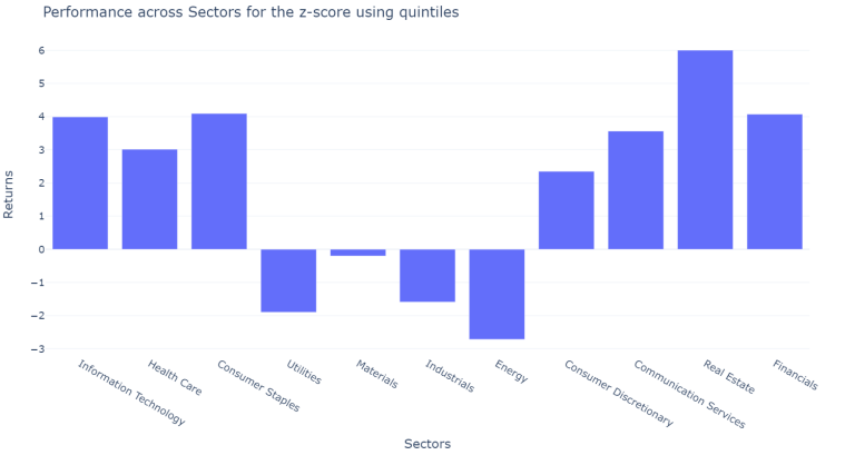
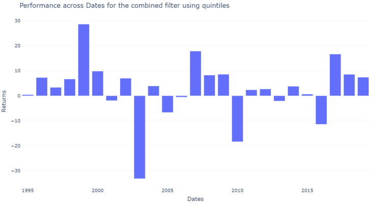
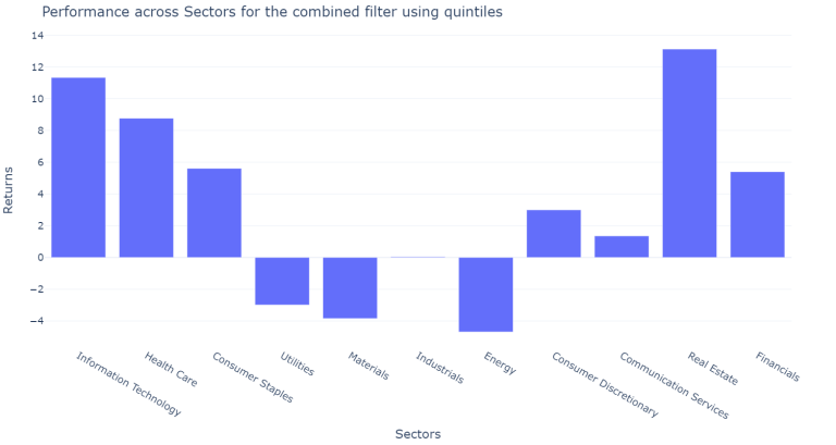
The results vary a lot across sectors and across years however our new filter performed slightly better than the previous combined filter. Neverthess, the individual filters still perform much better.
print("The average yearly result of the m-score is", round(100*df_m_only["results"].mean()), "BPS")
print("The average yearly result of the z-score is", round(100*df_z_only["results"].mean()), "BPS")
print("The average yearly result of the combined filter is", round(100*df_mix_only["results"].mean()), "BPS")
The average yearly result of the m-score is 24 BPS
The average yearly result of the z-score is 186 BPS
The average yearly result of the combined filter is 308 BPS
Using this new screening method, the results obtained are an average of 3.6 stocks for each sector for long screening as well as for short screening. Nevertheless, the companies in the long screening outperformed the companies in the short screening by 308 BPS more each year. Although, the filter is wrose than the previously defined screening method.
However, when we filter the stocks based on the quintiles for the m-score and the z-score alone, the results obtained are 24 and 1866 BPS more each year respectively.
The results across sectors using the new defined filter show that for the financial sector, which is most of the time excluded for studies based on the m-score and the z-score, the obtained results are over 500 BPS more return yearly for those banks fulfilling the criteria of the quintiles.
It is important to note, that the z-score was originally created for manufacturing companies. Altman later created a modified version of the z-score for companies that are not manufacturing and for emerging markets. However, the m-score obtained a much more stable performance across the years and across the sectors, only having a negative performance for the financial and the health care sector. This result is more consistent with part of the literature reviewed which excluded the financial sector to test the Beneish model, due to the differences on the financial ratios and the items off balance
4. Conclusions
The analysis performed for the constituents of the S&P500 from 1995 to 2020 exhibits positive results for both the m-score and the z-score as screening methods for the companies analysed. The combined model using the original cut-offs produces very few companies in the short screening. However, these companies are blue chips whose market capitalization is enormous, and their financial statements are constantly reviewed, thus it is not expected that many of them would be considered manipulators employing well known models such as the Beneish’s m-score. Still, both models are capable of selecting better performing stocks in the S&P500.
By screening the companies based on their relative m-score and z-score across sectors, the results of the screening method still perform well, producing better returns in the long screening than in the short screening. However, these results are worse than using the original numbers suggested by the authors for their models. It could be useful to add a measure of performance, instead of only looking at the probability of earnings manipulation and the probability of bankruptcy. Therefore, the companies could be filtered using a screening method and then ranked based on the performance. Nevertheless, this method could be more useful for companies in the long screening of the m-score model, as those in the short screening are more likely to have manipulated their earning and thus their reported performance would not be comparable across other companies.
Finally, the usefulness of the m-score and the z-score for investors are still relevant and they have produced positive results even years after their publication. Still, it is crucial to remember that this analysis made some assumptions explained in 3 Model definition, data and analysis.
Future lines of work
The imbalanced number of stocks after the screening method using the original cut-offs for the constituents of the S&P500 could be further expanded to smaller companies which might result in a more balanced dataset.
Moreover, the financial statements could be adjusted to improve comparability across companies, given the flexibility of accounting choices. In addition, when comparing companies reporting under different standards such as the IFRS and the US GAAP there are multiple differences that could be taken into consideration before computing the z-score and the m-score.
Another approach for detecting financial fraud was carried out with support vector machines and ensemble methods for US companies from 1991 to 2005 obtaining better performance than the Beneish model, using 24 raw financial variables instead of ratios (Li et al., 2015). This result is very promising, and the use of machine learning could be implemented to carry out the analysis as a method for screening stocks. However, more data would be needed as the dataset for that study contained more than 100.000 data points for different firms.
Finally, previous financial statements could be employed to carry out the analysis, the m-score included the previous year financial statements, nevertheless, another approach for screening could include previous m-scores in the calculation or even a feature containing the historical highest probability of earnings manipulation of a company.
Bibliography
Adu-Gyamfi, M., 2020. Investigating Financial Statement Fraud in Ghana using Beneish M-Score: A Case of Listed Companies on the Ghana Stock Exchange (GSE). [SSRN Scholarly Paper] Rochester, NY: Social Science Research Network. Available at: https://papers.ssrn.com/abstract=3627689 [Accessed 31 Dec. 2020].
Akra, R.M. and Chaya, J.K., 2020. Testing the Effectiveness of Altman and Beneish Models in Detecting Financial Fraud and Financial Manipulation: Case Study Kuwaiti Stock. International Journal of Business and Management, 15(10), p.70. Alfian, F. and Triani, N.N.A., 2018. FRAUDULENT FINANCIAL REPORTING DETECTION USING BENEISH M-SCORE MODEL IN PUBLIC COMPANIES IN 2012-2016. p.16.
Altman, E.I., 1968. FINANCIAL RATIOS, DISCRIMINANT ANALYSIS AND THE PREDICTION OF CORPORATE BANKRUPTCY. The Journal of Finance, 23(4), pp.589–609.
Anning, A.A. and Adusei, M., 2020. An Analysis of Financial Statement Manipulation among Listed Manufacturing and Trading Firms in Ghana. Journal of African Business, 0(0), pp.1–15. Beneish, M.D., Lee, C., Press, E., Whaley, B., Zmijewski, M. and Cisilino, P., 1999. The detection of earnings manipulation. Financial Analysts’ Journal, pp.24–36.
Dreyer CFA, C., 2020. The End of Accounting? Sustaining Financial Reporting. [online] CFA Institute Enterprising Investor. Available at: https://blogs.cfainstitute.org/investor/2020/12/30/the-end-of-accounting-sustaining-financial-reporting/ [Accessed 1 Jan. 2021].
Hakami, T., Rahmat, M.M., Yaacob, M.H. and Saleh, N.M., 2020. Fraud Detection Gap between Auditor and Fraud Detection Models: Evidence from Gulf Cooperation Council. Asian Journal of Accounting and Governance, 13(0), pp.1–13.
Hołda, A., 2020. Using the Beneish M-score model: Evidence from non-financial companies listed on the Warsaw Stock Exchange. Investment Management and Financial Innovations, 17(4), pp.389–401.
Kamal, M.E.M., Salleh, M.F.M. and Ahmad, A., 2016. Detecting Financial Statement Fraud by Malaysian Public Listed Companies: The Reliability of the Beneish M-Score Model. Jurnal Pengurusan (UKM Journal of Management), [online] 46(0). Available at: https://ejournal.ukm.my/pengurusan/article/view/8601 [Accessed 31 Dec. 2020].
Li, B., Yu, J., Zhang, J. and Ke, B., 2015. Detecting Accounting Frauds in Publicly Traded U.S. Firms: A Machine Learning Approach. p.16.
Mihalcea, M.-M., 2020. Detecting the Risk of Manipulation of Financial Statements for Companies on the Bucharest Stock Exchange Applying the Beneish Model. LUMEN Proceedings, 13, pp.182–193.
Özcan, A., 2018. The Use of Beneish Model in Forensic Accounting: Evidence from Turkey. p.11.
Papa CFA, V.P.P., CPA, FSA, 2018. The End of Accounting? Not So Sure. [online] CFA Institute Market Integrity Insights. Available at: https://blogs.cfainstitute.org/marketintegrity/2018/02/01/the-end-of-accounting-not-so-sure/ [Accessed 1 Jan. 2021].
Taherinia, M. and Talebi, R., 2019. ABILITY OF FRAUD TRIANGLE, FRAUD DIAMOND, BENEISH M SCORE, AND ALTMAN Z SCORE TO PREDICT FINANCIAL STATEMENTS FRAUD. p.14.