

Raksina Samasiri
Developer Advocate
Developer Advocate
Introduction
Inflation charts are everywhere - economic reports, dashboards, and news updates.
But even with all that data, I kept running into the same problem: It’s surprisingly hard to compare how inflation is evolving across multiple countries over time.
Line charts become cluttered with too many series. Tables provide precision but lack intuitive insight. So instead of searching for the “perfect dashboard,” I decided to build one.
In this article, I’ll walk through how to use LSEG Datastream with Python to create a global inflation dashboard using:
- Line charts (to understand trends)
- Heatmaps (to identify patterns)
Prerequisites
Before getting started, make sure you have the following:
- Python Environment: Python 3.8 or above (I'm using Python 3.12.12)
- Required Libraries: Install the required Python packages
- DatastreamPy==2.0.30
- pandas==3.0.3
- seaborn==0.13.2
- matplotlib==3.10.9
- Access to LSEG Datastream: You need valid Datastream credentials to run the examples.
- Basic Knowledge: Familiarity with basic scripting in Python
How to Use Datastream Navigator (Quick Guide)
Here’s a simple workflow based on the screenshots below.
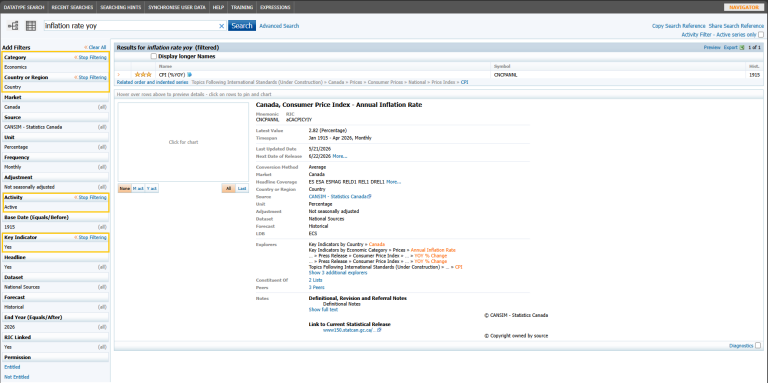
- Search for a Concept: In the search bar, enter a keyword like "inflation rate yoy". This returns multiple matching datasets.
- Apply Filters: On the left panel, remove irrelevant datasets quickly, narrow your results to:
- Category -> Economics
- Country or Region -> Region
- Activity -> Active
- Key Indicator -> Yes
- Inspect a Dataset: Click on a result to view its details.
From the image: These tell you that this is inflation that is expressed in percentage and updated regularly- Name: CPI (%YoY)
- Symbol: CNCPANNL
- Unit: Percentage
- Frequency: Monthly
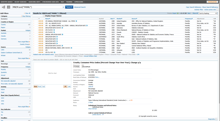
4. Identify Naming Patterns: Looking at multiple results:
- USCPANNL -> United States
- UKCPANNL -> United Kingdom
- JPCPANNL -> Japan
- CNCPANNL -> Canada
- Which you can infer a pattern: <Country Code> + CPANNL
5. Scale Your Dataset: Once you identify the pattern, you can build a dataset quickly. No need to manually search each country individually.
Important Note on Frequency
Although the Navigator shows Monthly Frequency . In practice, some macroeconomic datasets may behave like bi‑monthly observations (i.e. values not updated every single month), which means that the data points may appear every ~2 months. For visualization, treat it as time series (chronological order matters) and adjust display density as needed (e.g. every 4 months)
Step 1: Import Libraries Connect to DataStream
Import necessary Python library and initialize the Datastream client to query the data.
# Step 1: Import libraries and connect to DataStream
import DatastreamPy as dsws
import matplotlib.pyplot as plt
import seaborn as sns
import pandas as pd
ds=dsws.DataClient(username='YOUR_USERNAME',password='YOUR_PASSWORD')
Step 2: Define Countries
Define a list of inflation series across developed and emerging markets. Here we include a mix of developed and emerging markets:
# Step 2: Define Countries
series = [
"USCPANNL", # United States
"UKCPANNL", # United Kingdom
"JPCPANNL", # Japan
"FRCPANNL", # France
"ITCPANNL", # Italy
"DECPANNL", # Germany
"CNCPANNL", # Canada
"IDCPANNL", # Indonesia
"INCPANNL", # India
"NZCPANNL" # New Zealand
]
tickers_input = ",".join(series)
tickers_input

Step 3: Fetch Data
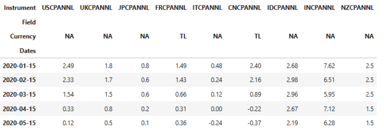
Retrieve time series data (bi‑monthly inflation observations). Datastream returns data in a wide format, where:
- rows = time (bi-monthly)
- columns = instruments
# Step 3: Fetch Data
data = ds.get_data(
tickers=tickers_input,
start="2020-01-01",
end="2026-01-01",
freq="M"
)
data.head()
Step 4: Clean and Standardize
Before visualization, we clean the dataset once as below - and reuse it everywhere.
- Convert index to datetime
- Sort by time
- Flatten column structure (returned data is in tuples for this ticker)
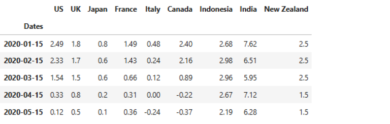
- To make the output readable, replace technical mnemonics with readable country names.
# Step 4: Clean and Standardize
df = data.copy()
# ensure datetime index
df.index = pd.to_datetime(df.index)
# sort by date
df = df.sort_index()
# FIX: columns from tuple to ticker string
df.columns = [c[0] if isinstance(c, tuple) else c for c in df.columns]
# map country names
country_map = {
"USCPANNL": "US",
"UKCPANNL": "UK",
"JPCPANNL": "Japan",
"FRCPANNL": "France",
"ITCPANNL": "Italy",
"DECPANNL": "Germany",
"CNCPANNL": "Canada",
"IDCPANNL": "Indonesia",
"INCPANNL": "India",
"NZCPANNL": "New Zealand"
}
df.columns = [country_map.get(c, c) for c in df.columns]
df.head()
Step 5: Visualizing Trends with Line Charts
Line chart helps identify global trends over time.
# Step 5: Visualizing Trends with Line Charts
df.plot(figsize=(18, 6))
plt.title("Global Inflation Trends (YoY %)")
plt.xlabel("Date")
plt.ylabel("Inflation (%)")
plt.legend(bbox_to_anchor=(1, 1), loc='upper left')
plt.grid(alpha=0.3)
plt.tight_layout()
plt.show()
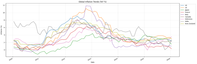
What this shows?
- A global inflation surge (2021–2022)
- A cooling trend (2023 onward)
- Differences across economies:
- Japan -> low inflation
- India -> persistently higher inflation
Step 6: Reusable Heatmap Functions
To make the visualization flexible, we separate:
- data preparation
- visualization
Step 6.1: Prepare Heatmap Data
- Transpose data (countries -> rows)
- Adjust frequency (bi‑monthly vs every 4 months)
- Format time labels
# Step 6.1: Prepare Heatmap Data
def prepare_heatmap_data(df, freq="bi-monthly"):
heatmap_df = df.T.copy()
# convert datetime
heatmap_df.columns = pd.to_datetime(heatmap_df.columns)
if freq == "reduced":
heatmap_df = heatmap_df.iloc[:, ::2] # every 4 months
# format date
heatmap_df.columns = heatmap_df.columns.strftime("%Y-%m")
return heatmap_df
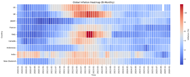
Step 6.2: Plot Heatmap
Heatmaps reveal cross-country patterns more clearly than line charts.
# Step 6.2: Plot Heatmap
def plot_inflation_heatmap(df, name):
plt.figure(figsize=(16, 6))
sns.heatmap(
df,
cmap="coolwarm",
linewidths=0.1,
cbar_kws={"label": "Inflation (%)"}
)
plt.title(name)
plt.xlabel("Time")
plt.ylabel("Country")
plt.tight_layout()
plt.show()
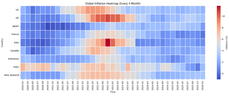
Step 6.3: Bi-Monthly vs Reduced Views
- Bi‑monthly: detailed view
- Every 4 months: cleaner comparison
# monthly
hm_monthly = prepare_heatmap_data(df, freq="bi-monthly")
plot_inflation_heatmap(hm_monthly, "Global Inflation Heatmap (Bi-Monthly)")
# quarterly
hm_quarterly = prepare_heatmap_data(df, freq="reduced")
plot_inflation_heatmap(hm_quarterly, "Global Inflation Heatmap (Every 4 Month)")
Why This Approach Works
A few key design decisions make this workflow effective:
- Use the right metric: Avoid unnecessary transformations by using inflation YoY directly
- Clean once, reuse everywhere: Mapping and formatting done early -> simpler downstream code
- Separate transformation from visualization: This enables flexible experimentation and reusable plotting functions
- Choose the right visualization
- Line charts -> trend over time
- Heatmaps -> cross-country comparison
Key Insights
From these visualizations:
- Inflation peaked globally around 2022
- Developed economies show similar patterns
- Emerging markets exhibit:
- higher baseline inflation
- slower normalization
Takeaways for Developers
If you're building data visualizations:
- Think about data structure first
- Choose the right metric, not just available data
- Clean once, reuse across visualizations
- Match the chart type to the question
Conclusion
This project wasn’t just about building a dashboard. It was about making global data easier to understand. Often, the biggest improvement in visualization doesn’t come from better charts, but from better thinking about the data.
- Register or Log in to applaud this article
- Let the author know how much this article helped you
If you require assistance, please
contact us here
Get In Touch
Source Code
Related Articles
Related APIs
Request Free Trial
Call your local sales team
Americas
All countries (toll free): +1 800 427 7570
Brazil: +55 11 47009629
Argentina: +54 11 53546700
Chile: +56 2 24838932
Mexico: +52 55 80005740
Colombia: +57 1 4419404
Europe, Middle East, Africa
Europe: +442045302020
Africa: +27 11 775 3188
Middle East & North Africa: 800035704182
Asia Pacific (Sub-Regional)
Australia & Pacific Islands: +612 8066 2494
China mainland: +86 10 6627 1095
Hong Kong & Macau: +852 3077 5499
India, Bangladesh, Nepal, Maldives & Sri Lanka:
+91 22 6180 7525
Indonesia: +622150960350
Japan: +813 6743 6515
Korea: +822 3478 4303
Malaysia & Brunei: +603 7 724 0502
New Zealand: +64 9913 6203
Philippines: 180 089 094 050 (Globe) or
180 014 410 639 (PLDT)
Singapore and all non-listed ASEAN Countries:
+65 6415 5484
Taiwan: +886 2 7734 4677
Thailand & Laos: +662 844 9576