

Raksina Samasiri
Developer Advocate
Learn how to retrieve historical vessel position snapshots from the Vessel Tracking API and visualize vessel positions on a world map using Python. In this tutorial, we'll call the API directly, process AIS position data, create a route visualization using Cartopy, and generate an animated playback showing how a vessel moved over time. This article is Part 1 of a two-part series, laying the foundation for real-time vessel tracking with WebSocket streaming.
AIS (Automatic Identification System) is a maritime tracking technology that enables vessels to broadcast their position and voyage information. The Vessel Tracking API makes this AIS data available for integration into custom applications and workflows.
Introduction
Maritime organizations rely heavily on vessel location data to monitor fleets, understand vessel positions, and support operational decision-making. However, raw AIS position reports containing latitude and longitude values can be difficult to interpret when viewed in tabular form.
Visualizing vessel positions on a map helps transform raw AIS position records into meaningful insights. A route visualization can reveal voyage patterns, identify changes in direction, highlight areas of activity, and provide stakeholders with an intuitive view of vessel positions over time.
The Vessel Tracking API provides access to historical and real-time vessel location data, making it possible to build monitoring applications, operational dashboards, and maritime analytics solutions.
In this article, we'll use Python to retrieve historical vessel position data directly from the Vessel Tracking API and transform it into both a static route visualization and an animated playback of a vessel's journey.
By the end of this tutorial, you'll be able to transform historical AIS position snapshots into a visual representation of a vessel's route and location history.
Note
- The /v1/Shipping/History endpoint provides access to the most recent 24 hours of vessel position history. If no FromDateTime and ToDateTime parameters are supplied, the API automatically returns data from the latest available 24-hour period.
- This is Part 1 of a two-part series. In Part 2, we'll consume streaming vessel position updates using WebSocket connections and visualize live vessel positions on a world map in near real time.
What We'll Build
In this article, we'll build a Python application that retrieves vessel position data from the Vessel Tracking API and creates an animated visualization of a vessel's route.
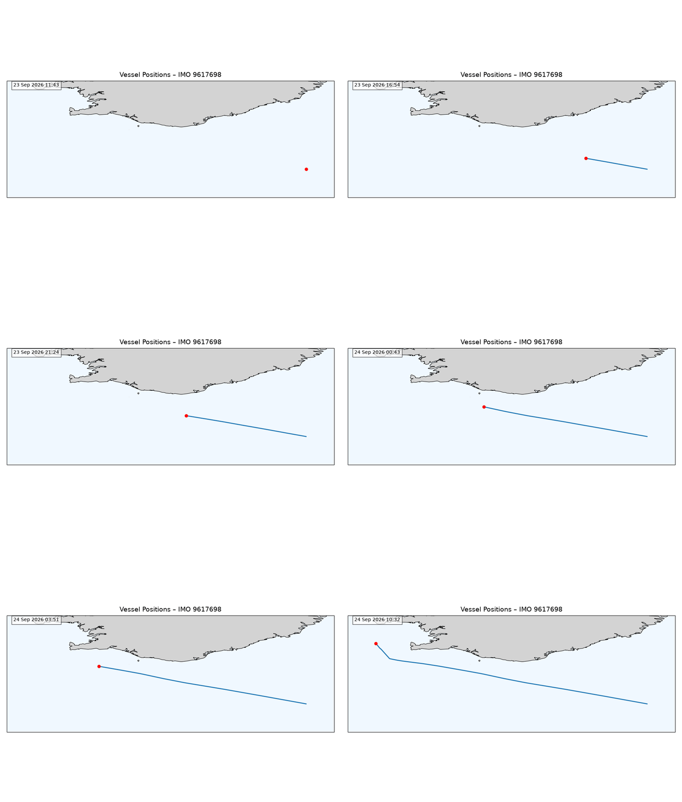
The final output looks similar to the animation below, the route is gradually drawn on a world map while the latest vessel position is highlighted and timestamped.
Why Visualize Vessel Routes?
AIS position data is commonly used for:
- Fleet monitoring
- Voyage analysis
- Vessel tracking
- Port and terminal operations
- Maritime intelligence
- Supply chain monitoring
While tables and spreadsheets are useful for analysis, they rarely provide an intuitive understanding of how a vessel actually moved.
Consider the following snapshot records:
| Timestamp | Latitude | Longitude |
| 2026-09-22 03:31 | 60.8225 | -1.2713 |
| 2026-09-22 03:42 | 60.8312 | -1.2561 |
| 2026-09-22 03:53 | 60.8452 | -1.2443 |
Although the data is technically complete, it can be difficult to identify:
- where the vessel is travelling
- how quickly it is moving
- whether it changed direction
- what route it followed
By plotting these positions on a map, the vessel's journey becomes immediately visible.
Prerequisites
Before getting started, make sure you have the following:
- Python 3.10 or later
- Python environment with the Jupyter Notebook extension and these libraries installed
- pandas==2.2.3
- requests==2.32.3
- matplotlib==3.10.0
- Cartopy==0.24.1
- Pillow==11.1.0
- IPython==8.31.0
- A Vessel Tracking API key
This tutorial assumes basic familiarity with Python and Jupyter Notebooks. We'll use Jupyter notebook and visualize the results.
If you don't already have a Vessel Tracking API key, contact your LSEG account representative or refer to the Vessel Tracking API documentation for instructions on generating one from the Vessel Tracking web application.
Solution Overview
In this example we'll use the Vessel Tracking API's History endpoint to retrieve historical vessel positions, process the returned AIS data using Pandas, and then visualize the route using Cartopy and Matplotlib.
The overall workflow looks like this::
Vessel Tracking API |
The final output will be a map showing the vessel's route as well as an animated replay of the vessel's positions over time.
Retrieving Historical Vessel Positions
This example retrieves data directly from the Vessel Tracking API using the History endpoint: GET /v1/Shipping/History
This endpoint is designed to retrieve recent position history for an individual vessel identified by an IMO, RIC, or ENI.
Understanding the Available History Window
One important characteristic of the History endpoint is that it only provides access to the most recent 24 hours of vessel position data.
At the time of writing:
- Historical data is limited to the latest available 24-hour period.
- If FromDateTime and ToDateTime are not specified, the API automatically returns the most recent 24 hours of available vessel positions.
- Requests for data older than the available 24-hour history window will not return results because the data is no longer available through this endpoint.
For example, if the latest available data covers: 22 Sep 2026 09:00 UTC to 23 Sep 2026 09:00 UTC
And a request is made using a FromDateTime earlier than the available history window, the API will be unable to return the requested records since they are no longer retained by the endpoint.
This behavior makes the History endpoint particularly useful for:
- Replaying recent vessel activity
- Investigating a voyage over the last day
- Visualizing recent positions
- Operational monitoring over the previous day
For longer-term historical analysis, developers should ensure that retrieved data is stored before it ages out of the endpoint's retention window.
For this example, we use an IMO number to retrieve vessel positions and the Python code converts the returned JSON response into a Pandas DataFrame for analysis and visualization.
# Vessel Tracking API configuration
BASE_URL = "https://vtracking.rdms.refinitiv.com/api/v1"
# In the full code example, we retrieve the API KEY from the configuration file named 'config.ini'. See the full example code in the repository linked on the top right of this article
API_KEY = 'YOUR_API_KEY_HERE'
if not API_KEY:
raise RuntimeError(
"Set the VESSEL_TRACKING_API_KEY environment variable with your "
"Vessel Tracking API key before running this notebook."
)
HEADERS = {"Authorization": API_KEY, "Accept": "application/json"}
# Vessel and date range to retrieve (History only accepts a single IMO/RIC/ENI per call)
IMO = 9617698
params = {"IMO": IMO}
# Optional date range:
# params["FromDate"] = "2026-04-30T00:00:00Z"
# params["ToDate"] = "2026-04-30T23:59:59Z"
response = requests.get(
f"{BASE_URL}/Shipping/History",
params=params,
headers=HEADERS,
timeout=30,
)
response.raise_for_status()
# Each record comes back as {"fieldNames": [...], "fieldValues": [...]} rather than
# a flat object, so zip the two arrays together to get real column names.
records = response.json()
rows = [dict(zip(record["fieldNames"], record["fieldValues"])) for record in records]
df = pd.DataFrame(rows)
# All values arrive as strings, so cast the columns we do math/comparisons on to numbers.
df["IMO"] = pd.to_numeric(df["IMO"], errors="coerce")
df["Latitude"] = pd.to_numeric(df["Latitude"], errors="coerce")
df["Longitude"] = pd.to_numeric(df["Longitude"], errors="coerce")
df.head()
# Take a quick look at the retrieved data
Understanding the Returned Data
The Vessel Tracking API can return a rich set of vessel attributes, including:
| Field | Description |
|---|---|
| Latitude / Longitude | Current vessel position |
| SpeedOverGround | Reported vessel speed |
| Heading | Current heading |
| NavigationalStatus | Operational status of the vessel |
| AISDestination | Destination reported through AIS |
| EstTimeOfArrival | Estimated arrival time |
In this article, we'll focus primarily on latitude, longitude, and timestamp fields for visualization purposes.
Preparing the Dataset
Before visualizing the route, we need to ensure that the data is suitable for plotting.
AIS datasets occasionally contain:
- Missing coordinates
- Missing timestamps
- Invalid values
- Incomplete records
Those records cannot be plotted on a map and therefore need to be removed.
We also convert timestamps into Python datetime objects so that the route can be sorted chronologically and displayed correctly during the animation.
After preparing the dataset, we can inspect some summary statistics:
| Row count: 106 Date range: 2026-09-21 20:31:47 to 2026-09-22 09:24:06 |
This quick validation step helps confirm that data has been retrieved successfully and that the expected position history is available.
# Drop rows without valid coordinates or a timestamp — required for plotting
df = df.dropna(subset=["Latitude", "Longitude", "TimestampPosition"])
# Convert the timestamp column from text to a proper datetime type.
# The API returns timestamps in ISO-like "YYYY-MM-DD HH:MM:SS" format.
# errors="coerce" turns any unparseable values into NaT instead of raising an error.
df["TimestampPosition"] = pd.to_datetime(
df["TimestampPosition"],
errors="coerce"
)
# Drop any rows where the timestamp failed to parse
df = df.dropna(subset=["TimestampPosition"])
# Quick summary of the cleaned dataset
print(f"Row count : {len(df)}")
print(f"Date range : {df['TimestampPosition'].min()} to {df['TimestampPosition'].max()}")
print(f"Number of IMOs : {df['IMO'].nunique()}")
Selecting a Vessel
For this walkthrough we focus on a single vessel: IMO = 9617698
The retrieved positions are sorted chronologically so that the route follows the same order in which the vessel travelled.
To create smoother playback, the notebook also reduces the number of plotted points by keeping every third AIS record with: .iloc[::3]
This approach:
- Reduces the total number of animation frames
- Improves playback performance
- Preserves the overall shape of the route
# IMO was already used to scope the API request above; re-filter here as a safety net
track = (
df[df["IMO"] == IMO]
.sort_values("TimestampPosition")
.iloc[::3] # thin points for smoother, faster playback
.reset_index(drop=True)
)
print(f"Number of position points for IMO {IMO}: {len(track)}")
track.head()
Creating a Static Route Visualization
Before creating an animation, it's often useful to inspect the complete route on a static map.
Using Cartopy allows us to render:
- oceans
- coastlines
- countries
- land masses
providing geographical context around the vessel's positions.
Route Visualization
# A small margin around the route's bounding box, in degrees
pad = 1
fig = plt.figure(figsize=(9, 12))
ax = plt.axes(projection=ccrs.PlateCarree())
ax.set_extent(
[
track["Longitude"].min() - pad,
track["Longitude"].max() + pad,
track["Latitude"].min() - pad,
track["Latitude"].max() + pad,
],
crs=ccrs.PlateCarree(),
)
# Real-world basemap layers
ax.add_feature(cfeature.LAND, facecolor="lightgrey")
ax.add_feature(cfeature.OCEAN, facecolor="aliceblue")
ax.add_feature(cfeature.COASTLINE, linewidth=0.8)
ax.add_feature(cfeature.BORDERS, linestyle=":", linewidth=0.6)
ax.set_title(f"Vessel Route \u2013 IMO {IMO}", fontsize=14)
ax.plot(
track["Longitude"], track["Latitude"],
marker="o", markersize=3, lw=1,
transform=ccrs.PlateCarree(),
)
plt.show()
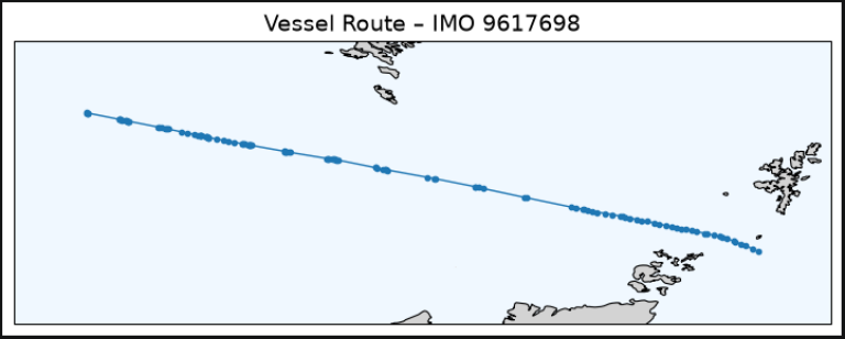
The route immediately reveals several pieces of information that would be difficult to infer from raw position records alone:
- the overall direction of travel
- the distance covered
- turning points along the voyage
- the vessel's latest known position
This type of visualization is often sufficient for quick operational reviews and voyage analysis.
Bringing the Route to Life
While the static route provides useful context, it does not reveal how the vessel moved over time.
To add a temporal dimension, we create an animated playback using Matplotlib's FuncAnimation.
The animation gradually:
- Draws the route line as time progresses.
- Moves a marker along the vessel's path.
- Displays the corresponding timestamp for each AIS position report.
This creates an effect similar to replaying the vessel's journey.
Animated Playback
# Figure setup — dynamically size the canvas based on the route's geographic bounds
# Add a small margin around the route, in degrees
pad = 1
# Calculate the geographic bounding box of the complete route
lon_min = track["Longitude"].min() - pad
lon_max = track["Longitude"].max() + pad
lat_min = track["Latitude"].min() - pad
lat_max = track["Latitude"].max() + pad
# Correct the longitude span for latitude to approximate the map's visual width
mean_lat = (lat_min + lat_max) / 2
map_width = (lon_max - lon_min) * np.cos(np.radians(mean_lat))
map_height = lat_max - lat_min
# Calculate and constrain the aspect ratio to avoid excessively wide or tall output
aspect_ratio = map_width / max(map_height, 0.01)
aspect_ratio = np.clip(aspect_ratio, 0.6, 2.5)
# Dynamically calculate the figure height while keeping its size within useful limits
figure_width = 10
figure_height = figure_width / aspect_ratio
figure_height = np.clip(figure_height, 4, 10)
# Let the map occupy most of the canvas to minimize surrounding whitespace
fig = plt.figure(figsize=(figure_width, figure_height))
ax = fig.add_axes(
[0.02, 0.03, 0.96, 0.90],
projection=ccrs.PlateCarree(),
)
# Display the complete route using its dynamically calculated bounds
ax.set_extent(
[lon_min, lon_max, lat_min, lat_max],
crs=ccrs.PlateCarree(),
)
ax.set_title(f"Vessel Positions – IMO {IMO}", fontsize=14, pad=8)
ax.add_feature(cfeature.LAND, facecolor="lightgrey")
ax.add_feature(cfeature.OCEAN, facecolor="aliceblue")
ax.add_feature(cfeature.COASTLINE, linewidth=0.8)
ax.add_feature(cfeature.BORDERS, linestyle=":", linewidth=0.6)
# The route line (drawn gradually) and the current-position marker
line, = ax.plot([], [], lw=2, transform=ccrs.PlateCarree())
point, = ax.plot([], [], "ro", markersize=6, transform=ccrs.PlateCarree())
# Text annotation showing the current timestamp
time_text = ax.text(
0.02, 0.95, "", transform=ax.transAxes,
fontsize=10, bbox=dict(facecolor="white", alpha=0.7)
)
def init():
"""Reset all animated artists to an empty state at the start of the animation."""
line.set_data([], [])
point.set_data([], [])
time_text.set_text("")
return line, point, time_text
def update(frame):
"""Draw the route up to the current frame and move the marker to the latest position."""
xs = track["Longitude"].iloc[:frame + 1]
ys = track["Latitude"].iloc[:frame + 1]
line.set_data(xs, ys)
point.set_data(xs.iloc[-1:], ys.iloc[-1:])
time_text.set_text(track["TimestampPosition"].iloc[frame].strftime("%d %b %Y %H:%M"))
return line, point, time_text
ani = FuncAnimation(
fig,
update,
frames=len(track),
init_func=init,
interval=80, # milliseconds between frames
repeat=False
)
plt.close(fig) # prevent a duplicate static plot from being displayed below the animation
The moving marker represents the vessel's current position, while the timestamp overlay indicates when each recorded position was observed.
This type of visualization is particularly useful when:
- demonstrating vessel positions to stakeholders
- investigating voyage behavior
- validating AIS datasets
- creating operational dashboards
Exporting the Animation
The completed animation can be exported as a GIF
This makes it easy to:
- share through email
- include in presentations
- embed in reports
- publish as part of web-based applications
The exported file also serves as a lightweight method for communicating vessel activity to non-technical audiences.
ani.save(
"IMO_9617698_Positions.gif",
writer="pillow"
)
Potential Enhancements
This example intentionally focuses on a single vessel to keep the workflow easy to understand.
In production environments, the same approach can be extended to support:
- Fleet Tracking: Track multiple vessels simultaneously on the same map.
- Port Monitoring: Visualize vessels approaching or departing ports.
- Trade Flow Analysis: Animate vessel locations across shipping lanes and regions.
- Geofencing: Highlight vessel activity within predefined areas.
- Operational Dashboards: Combine vessel positions with business workflows, alerts, and analytics.
Source Code
The complete source code and Jupyter Notebook used throughout this tutorial are available in the GitHub repository linked in the top-right corner of this page.
You can use the notebook as a starting point and adapt it to visualize different vessels, adjust the animation settings, or build more advanced maritime monitoring applications.
Conclusion
In this article, we demonstrated how historical AIS position data from the Vessel Tracking API can be transformed into an intuitive visual representation of vessel position.
Starting from a simple API request, we:
- Retrieved historical vessel positions
- Cleaned and prepared the dataset
- Visualized vessel routes on a world map
- Created an animated route playback
- Exported the animation as a GIF
While this example uses historical position snapshots from the previous 24 hours, the same techniques can be applied to more advanced maritime analytics and monitoring applications.
Next Steps: Moving to Real-Time Streaming
In this article, we replayed historical vessel positions using the History endpoint.
What if we wanted to see vessel positions update live as they are reported?
In Part 2 of this series, we'll connect to the Vessel Tracking WebSocket interface and build a near real-time vessel tracking application that:
- subscribes to vessel updates
- receives AIS position events as they occur
- updates a world map automatically
- provides the foundation for a live maritime monitoring dashboard
Instead of replaying history, we'll be visualizing vessel positions as they happen.
- Register or Log in to applaud this article
- Let the author know how much this article helped you
If you require assistance, please
contact us here
Get In Touch

Source Code
Related APIs
Related Articles
-
Check LSEG Data Library for Python Usage Limits Remaining
-
The Data Library for Python - Quick Reference Guide (Access layer)
-
Step-By-Step Guide to install Data Library for Python using Virtual Environment
-
LSEG Data Library for Python: News Pagination
-
LSEG’s Refinitiv Data Library for Python and its Configuration Process
Request Free Trial
Call your local sales team
Americas
All countries (toll free): +1 800 427 7570
Brazil: +55 11 47009629
Argentina: +54 11 53546700
Chile: +56 2 24838932
Mexico: +52 55 80005740
Colombia: +57 1 4419404
Europe, Middle East, Africa
Europe: +442045302020
Africa: +27 11 775 3188
Middle East & North Africa: 800035704182
Asia Pacific (Sub-Regional)
Australia & Pacific Islands: +612 8066 2494
China mainland: +86 10 6627 1095
Hong Kong & Macau: +852 3077 5499
India, Bangladesh, Nepal, Maldives & Sri Lanka:
+91 22 6180 7525
Indonesia: +622150960350
Japan: +813 6743 6515
Korea: +822 3478 4303
Malaysia & Brunei: +603 7 724 0502
New Zealand: +64 9913 6203
Philippines: 180 089 094 050 (Globe) or
180 014 410 639 (PLDT)
Singapore and all non-listed ASEAN Countries:
+65 6415 5484
Taiwan: +886 2 7734 4677
Thailand & Laos: +662 844 9576