

Every day, LSEG delivers thousands of Reuters News stories touching the energy sector — pipeline outages, refinery fires, OPEC production adjustments, conflict, sanctions, weather events, regulatory changes. For an analyst trying to build a systematic view of energy supply disruptions, the challenge is not volume; it is relevance.
A keyword search for "oil supply disruption" will return some useful stories — and a great deal of noise. This notebook demonstrates a different approach: using the structured classification metadata that Reuters News attaches to every story to define a precise, repeatable signal for energy supply disruptions.
The goal is not prediction. It is signal construction — turning an unstructured information flow into something that can be measured, filtered, and combined with other market data.
Setup
This notebook uses the LSEG Data Library for Python to retrieve news headlines and story content.
It also relies on a locally included helper package called newstokens, which provides a simple interface for interpreting the structured classification codes (QCodes) attached to news stories. Rather than working with raw code identifiers, this package resolves them into descriptive labels, navigates parent-child relationships, and extracts the metadata embedded within individual stories. It is used throughout this article to make the classification system readable and explorable.
The internals of newstokens are beyond the scope of this article — the source is included alongside the notebook for readers who wish to review the implementation details at their own convenience.
import lseg.data as ld
from lseg.data.content import news
from newstokens.tokens import tokens
from newstokens.tokens.enums import TokenCategory
import pandas as pd
import plotly.express as px
import plotly.graph_objects as go
import warnings
warnings.filterwarnings("ignore", category=FutureWarning, module="lseg")
pd.set_option("display.max_colwidth", 120)
# Establish communication with our LSEG data environment.
# Initialize the session - Desktop mode (Workspace)
ld.open_session()
Signal Definition
Before exploring the data, we define the structured codes that make up our energy supply disruption signal. Each code represents a classification dimension assigned to Reuters News stories — not a keyword, but a semantic label applied at publication time.
Centralizing these definitions here makes the signal explicit, easy to modify, and reusable across all queries in this notebook.
# Signal Definition
# These codes define the structured filter for energy supply disruptions.
# Each constant is a list so you can add or remove codes to adjust the signal.
ENERGY_SECTOR = ["B:219"] # Energy (TRBC level 1) — covers fossil fuels, renewables, uranium
SUPPLY_TOPICS = ["I:6K", "M:3D0", "M:2Z9"] # Commodity Production Data; Supply Chain Issues; FCA - Drilling / Production Report
MIDDLE_EAST = ["G:Q"] # Middle East geographic region
# Build reusable query fragments from the signal definition
sector_filter = " OR ".join(ENERGY_SECTOR)
topic_filter = " OR ".join(SUPPLY_TOPICS)
signal_query = f"({sector_filter}) AND ({topic_filter})"
print(f"Signal query: {signal_query}")
Signal query: (B:219) AND (I:6K OR M:3D0 OR M:2Z9)
Discovering Codes
But how were these codes identified? The newstokens helper provides a browse() method that lets you search within any taxonomy category using a server-side text query. For example, to find geographic codes related to the Middle East:
# Browse geographic tokens matching "Middle East"
tokens.browse(category=TokenCategory.GEOGRAPHIES, query="Middle East")

The browse() method supports several taxonomy categories — including BUSINESS_SECTORS, MARKETS, MORE_TOPICS, and others — and accepts a query parameter for server-side filtering. This makes it straightforward to explore the classification system and identify the codes you need for any signal definition. The codes used in this article were selected using exactly this kind of exploration.
1. The Problem with Keywords
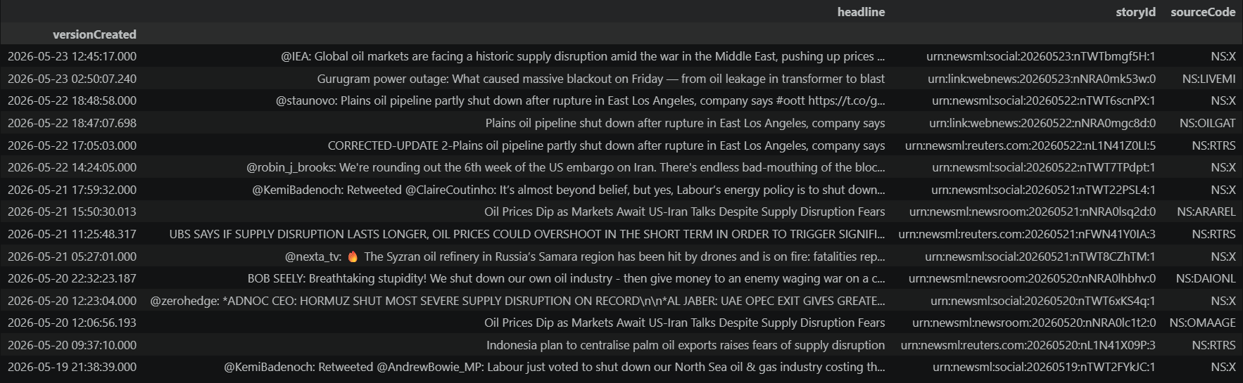
The most intuitive way to find news about energy supply disruptions is to search for them by keyword. Let's try that first and see what comes back.
# A broad keyword search for energy supply disruption stories
keyword_results = ld.news.get_headlines(
query='"oil" AND ("supply disruption" OR "outage" OR "shut down" OR "force majeure")',
count=50
)
keyword_results.head(15)
# Extract the source type from the storyId URN structure
# Format: urn:{scheme}:{source}:{date}:{id}:{version}
keyword_results['source'] = keyword_results['storyId'].str.split(':').str[2]
source_counts = keyword_results['source'].value_counts()
print("Story sources in keyword results:")
print(source_counts.to_string())
print(f"\nSocial media stories: {source_counts.get('social', 0)} of {len(keyword_results)} ({source_counts.get('social', 0) / len(keyword_results) * 100:.0f}%)")
Story sources in keyword results:
source
social 35
webnews 8
reuters.com 4
newsroom 3
Social media stories: 35 of 50 (70%)
At first glance, many of these headlines look relevant. But look closer — the storyId URN itself reveals important context. Its structure — urn:{scheme}:{source}:{date}:{id}:{version} — encodes the source type of each story. Parsing it shows that a significant portion of keyword results come from social sources (tweets, retweets, commentary on X/Twitter) rather than editorial news content.
This is a key insight: keyword searches don't just match irrelevant topics — they pull in entirely different content types. Social media posts that happen to contain the right words are returned alongside editorial reporting, with no built-in way to distinguish them. The breakdown above quantifies this noise.
Beyond social media, keyword search may also pull in:
- Commentary and opinion pieces that mention disruptions in passing
- Market roundups where supply is one of several themes discussed
- Downstream stories (demand-side, retail pricing) that happen to use supply-related language
- Unrelated sectors where similar vocabulary appears (e.g., power grid outages, supply chain logistics)
The fundamental issue is that keywords match language, not meaning. A story can use the word "disruption" without being about a supply disruption event. And a story about a pipeline explosion may never use the word "disruption" at all.
To build a reliable signal, we need something that captures what a story is about — not just what words it contains.
2. Defining the Signal with Structured Metadata
Every Reuters News story is classified at publication time with a set of structured codes. These codes describe the story's topic, industry sector, named entities, geography, and more. They are assigned by a combination of editorial rules and automated classification — not by keyword matching.
This means we can define our signal not as a bag of words, but as a combination of structured attributes that together describe what we care about: energy supply disruptions.
Let's start by identifying the relevant building blocks.
# What does the Energy sector look like in the classification system?
energy_sector = tokens.resolve(ENERGY_SECTOR)
energy_sector

# What sub-sectors exist under Energy?
energy_children = pd.concat([tokens.children(code) for code in ENERGY_SECTOR], ignore_index=True)
energy_children

The classification system organizes energy into meaningful sub-sectors — oil & gas, coal, renewables, nuclear, and so on. Rather than searching for the word "oil," we can target stories that have been classified as being about specific energy sub-sectors.
But sector alone is not enough. We also need to narrow by topic — specifically, supply-side disruption events.
# Identify supply-related topic codes
supply_topics = tokens.resolve(SUPPLY_TOPICS)
supply_topics

Now we have two dimensions of classification:
| Dimension | Purpose | Example Codes |
|---|---|---|
| Sector | What industry is the story about? | ENERGY_SECTOR — Energy and children |
| Topic | What kind of event is described? | SUPPLY_TOPICS — Supply/Demand, Output/Production |
By requiring both dimensions to be present, we can construct a much more precise filter than any keyword search can achieve. A story must be classified as energy-sector and classified as covering a supply-side event to pass through.
3. Retrieving the Signal
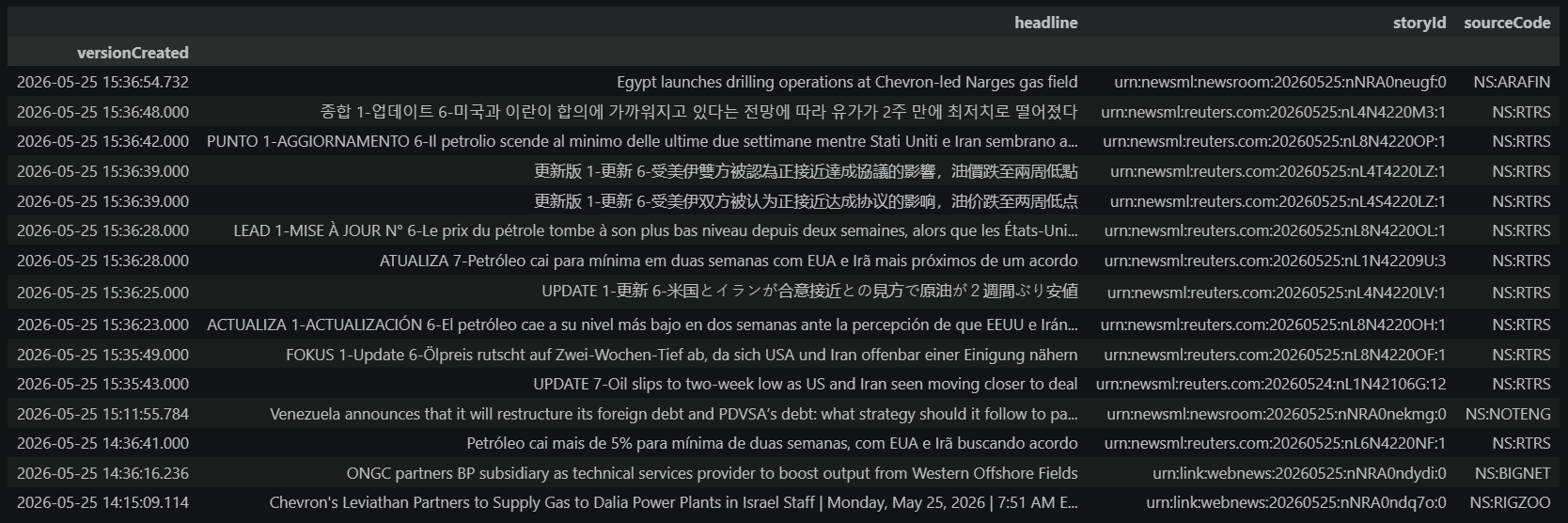
With our signal defined as an intersection of sector and topic classifications, we can now query for stories that match.
# Retrieve stories matching our signal definition
signal_results = ld.news.get_headlines(
query=signal_query,
count=50
)
print(f"Stories matching structured signal: {len(signal_results)}")
signal_results.head(15)
Stories matching structured signal: 50
# Apply the same URN source analysis to the structured signal results
signal_results['source'] = signal_results['storyId'].str.split(':').str[2]
signal_source_counts = signal_results['source'].value_counts()
print("Story sources in structured signal results:")
print(signal_source_counts.to_string())
print(f"\nSocial media stories: {signal_source_counts.get('social', 0)} of {len(signal_results)} ({signal_source_counts.get('social', 0) / len(signal_results) * 100:.0f}%)")
Story sources in structured signal results:
source
reuters.com 36
webnews 9
newsroom 4
social 1
Social media stories: 1 of 50 (2%)
Compare these source breakdowns with the keyword results in Section 1. The difference is striking: keyword search returned a mix of social, webnews, and newsroom content — with social media making up a large share. The structured signal, by contrast, is dominated by editorial sources. Social media posts simply don't carry the classification codes that the structured query requires, so they're filtered out by design.
This single comparison — parsing the storyId URN from both approaches — tells most of the story. The structured query doesn't just find better topics; it finds a fundamentally different class of content. No additional metadata inspection is needed to see that.
4. What's Inside a Story: Examining the Metadata
To understand why this approach works, it helps to look at the classification attached to an individual story. Each story carries a subject array of structured codes — the editorial classification that describes sector, topic, geography, and more. We can extract those raw codes and resolve them into human-readable descriptions using our metadata helper.
Note: Not every story will have subject codes populated at the time you retrieve it. Breaking or high-priority stories are often published immediately and may initially arrive with an empty subject_codes array. Metadata such as subject classifications can be added or updated after the initial publication, at which point the story may be re-published with the enriched data. If the story you select has no subject codes, simply try a different index (e.g., iloc[1] instead of iloc[0]) or choose another story ID from the results.
# Pick a story from our signal results
sample_story_id = signal_results.iloc[1]['storyId']
# Retrieve the story and extract its subject codes
story = news.story.Definition(sample_story_id).get_data()
s = story.data.story
subject_codes = s.subject_codes
# Show some of the raw codes to demonstrate what is available...
print(", ".join(subject_codes[:10]) + ", ...")
A:4, G:3, G:A, G:AE, G:Q, G:V, M:3F, U:24, U:45, U:C, ...
# Resolve the raw codes into readable descriptions
tokens.resolve(subject_codes)
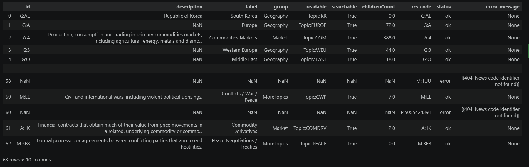
You'll notice that some rows in the table above show a status of error with the message "News code identifier not found". These are consistently codes that begin with P: — for example, P:50554244391. These are not classification codes at all; they are PermIDs (Permanent Identifiers), LSEG's system for uniquely identifying real-world entities such as companies, people, and organizations.
PermIDs appear in the subject array because it serves as a unified tagging container — it carries not only the editorial classification (topic, sector, geography) but also entity annotations that link the story to specific real-world entities. This is by design: it allows consumers of the data to connect a story to the broader LSEG entity ecosystem, where a PermID can be used to look up company fundamentals, ownership structures, or other reference data. Because our metadata helper only resolves news classification codes, PermIDs fall outside its scope and can be safely ignored here.
The raw codes on their own are opaque. But once resolved through the metadata API, they become a structured profile of the story: which sector it covers, what topics it addresses, which geographies are relevant, and more.
This is the key insight: every story carries a machine-readable description of what it is about, not just the words it contains. That depth of classification is what allows us to build precise filters. And because it's applied consistently across all stories, the signal is repeatable — the same query run tomorrow will apply the same logic to new stories.
The newstokens helper also provides a convenience method — tokens.resolve_story(story_id) — that wraps the extraction and resolution steps above into a single call. We'll use it later when processing multiple stories at once.
5. Sharpening the Signal: Adding Geographic Focus
Our current signal captures energy supply stories globally. Depending on the use case, we may want to narrow further — for example, focusing on supply disruptions in a specific producing region.
Structured metadata makes this straightforward. We simply add a geographic dimension to our filter.
# Look up the geographic code for our regional focus
geo_codes = tokens.resolve(MIDDLE_EAST)
geo_codes

# Narrow the signal to Middle East energy supply disruptions
geo_filter = " OR ".join(MIDDLE_EAST)
regional_query = f"{signal_query} AND ({geo_filter})"
regional_results = ld.news.get_headlines(
query=regional_query,
count=50
)
print(f"Middle East energy supply stories: {len(regional_results)}")
regional_results.head(10)
Middle East energy supply stories: 50
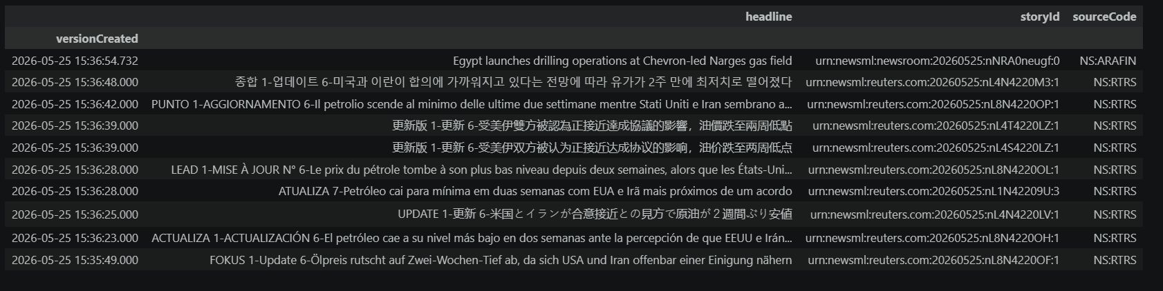
Each additional metadata dimension we layer in increases precision without sacrificing the systematic nature of the approach. We could further refine by:
- Sub-sector: Narrow to crude oil vs. natural gas vs. LNG
- Event type: Distinguish planned maintenance from unplanned outages
- Named entities: Focus on specific companies or facilities
The key insight is that these refinements are compositional — you build them by combining structured codes, not by inventing more complex keyword patterns.
6. Confirming the Difference Over a Common Window
The source breakdowns in Sections 1 and 3 already reveal the core difference: keyword search mixes social media, web aggregation, and editorial content indiscriminately, while the structured signal is inherently filtered to classified, editorial stories. To confirm this holds consistently, we can run both approaches over the same one-month window and compare their source composition side by side.
This also lets us check for blind spots — stories the structured signal captures that keyword search misses entirely, because the relevant events were described in language the keyword pattern doesn't anticipate.
# Retrieve both sets over the same one-month window
today = pd.Timestamp.now().normalize()
date_from = (today - pd.DateOffset(months=1)).strftime("%Y-%m-%d")
date_to = today.strftime("%Y-%m-%d")
keyword_month = ld.news.get_headlines(
query='"oil" AND ("supply disruption" OR "outage" OR "shut down" OR "force majeure")',
start=date_from,
end=date_to,
count=100
)
structured_month = ld.news.get_headlines(
query=signal_query,
start=date_from,
end=date_to,
count=100
)
# Compare source composition side by side
keyword_month['source'] = keyword_month['storyId'].str.split(':').str[2]
structured_month['source'] = structured_month['storyId'].str.split(':').str[2]
kw_sources = keyword_month['source'].value_counts()
st_sources = structured_month['source'].value_counts()
comparison = pd.DataFrame({
'Keyword Search': kw_sources,
'Structured Signal': st_sources
}).fillna(0).astype(int)
print(f"Source comparison over {date_from} to {date_to}\n")
print(comparison.to_string())
print(f"\nKeyword total: {len(keyword_month)} | Structured total: {len(structured_month)}")
print(f"Keyword social: {kw_sources.get('social', 0)} ({kw_sources.get('social', 0) / len(keyword_month) * 100:.0f}%) | Structured social: {st_sources.get('social', 0)} ({st_sources.get('social', 0) / len(structured_month) * 100:.0f}%)")
# Check for blind spots — stories structured signal found that keywords missed
keyword_story_ids = set(keyword_month['storyId'])
structured_only = structured_month[~structured_month['storyId'].isin(keyword_story_ids)]
if len(structured_only) > 0:
print(f"\n--- Structured signal results missed by keywords ({len(structured_only)} of {len(structured_month)}) ---")
for _, row in structured_only.head(5).iterrows():
print(f" • {row['headline']}")
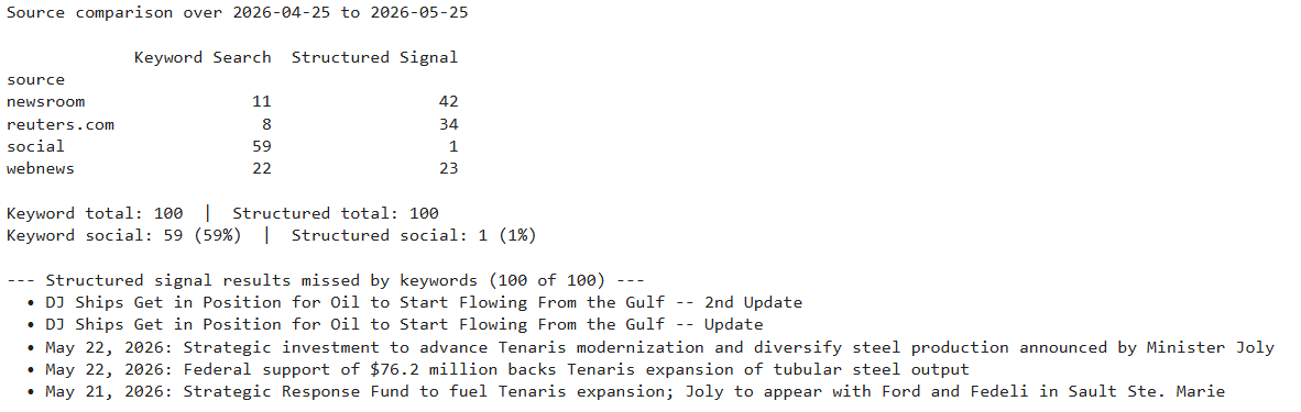
The side-by-side source comparison confirms what Sections 1 and 3 already suggested: keyword search pulls in a large share of social media and aggregated web content, while the structured signal is composed almost entirely of editorially classified stories. The blind spots list further illustrates that keywords miss genuine supply events when the story uses different vocabulary.
This is the core value of the structured approach: it filters by meaning, not language — and in doing so, it eliminates entire categories of noise (social media, opinion, off-topic mentions) that keyword search cannot distinguish from relevant editorial reporting.
7. Measuring the Signal Over Time
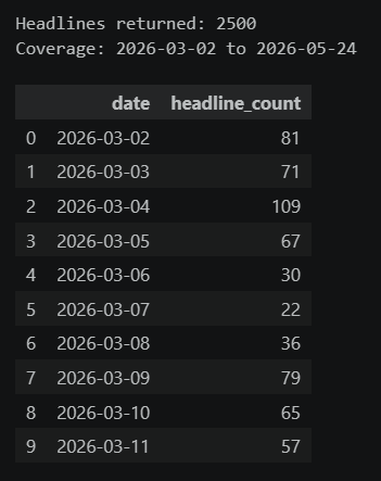
Once we have a clean, well-defined signal, we can measure it. A simple but useful metric is headline frequency — how many disruption-related headlines are being published per day? Spikes in frequency often correspond to real-world events.
# Retrieve a broader window for time-series analysis
today = pd.Timestamp.now().normalize()
three_months_ago = (today - pd.DateOffset(months=3)).strftime("%Y-%m-%d")
today_str = today.strftime("%Y-%m-%d")
signal_extended = ld.news.get_headlines(
query=regional_query,
start=three_months_ago,
end=today_str,
count=2500
)
# Build a daily frequency series
signal_extended['date'] = pd.to_datetime(signal_extended.index).normalize().tz_localize(None)
daily_counts = signal_extended.groupby('date').size().reset_index(name='headline_count')
# Reindex only over the range actually covered by the returned headlines.
# The API returns the most recent N headlines (count=500), so earlier dates in the
# requested window may have no coverage — filling those with zero would be misleading.
actual_start = signal_extended['date'].min()
actual_end = signal_extended['date'].max()
daily_counts = daily_counts.set_index('date').reindex(
pd.date_range(actual_start, actual_end), fill_value=0
).rename_axis('date').reset_index()
print(f"Headlines returned: {len(signal_extended)}")
print(f"Coverage: {actual_start.strftime('%Y-%m-%d')} to {actual_end.strftime('%Y-%m-%d')}")
daily_counts.head(10)
# Add a rolling average to smooth daily volatility
daily_counts['rolling_7d'] = daily_counts['headline_count'].rolling(window=7, min_periods=1).mean()
fig = go.Figure()
fig.add_trace(go.Bar(
x=daily_counts['date'],
y=daily_counts['headline_count'],
name='Daily Headline Count',
marker_color='lightsteelblue',
opacity=0.6
))
fig.add_trace(go.Scatter(
x=daily_counts['date'],
y=daily_counts['rolling_7d'],
name='7-Day Rolling Average',
line=dict(color='#636EFA', width=2.5)
))
fig.update_layout(
title='Energy Supply Disruption Signal: Daily Headline Frequency',
xaxis_title='Date',
yaxis_title='Number of Headlines',
template='plotly_white',
legend=dict(yanchor='top', y=0.99, xanchor='right', x=0.99)
)
fig.show()
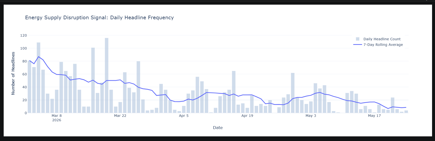
Spikes in the signal typically correspond to real-world disruption events — a refinery outage, sanctions escalation, weather-driven supply interruptions, or OPEC production decisions. The structured approach ensures these spikes reflect actual supply events, not just increased use of disruption-related vocabulary in broader market coverage.
8. From Signal to Context: What's Driving the Spike?
The chart above shows daily headline frequency over the coverage window. Some days have noticeably higher counts than others — these are the "spikes." But a spike on its own only tells us when disruption coverage intensified, not why.
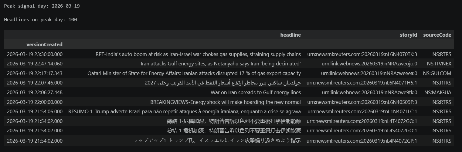
To answer that, we take the peak day — the single date with the highest headline count — and decompose its metadata. By examining which classification codes appear most frequently across that day's headlines, we can identify the sub-sectors, geographies, and topics that drove the surge.
# Find the peak day
peak_day = daily_counts.loc[daily_counts['headline_count'].idxmax(), 'date']
print(f"Peak signal day: {peak_day.strftime('%Y-%m-%d')}")
# Retrieve headlines from the peak day
peak_headlines = ld.news.get_headlines(
query=regional_query,
start=peak_day.strftime('%Y-%m-%d'),
end=(peak_day + pd.Timedelta(days=1)).strftime('%Y-%m-%d'),
count=100
)
print(f"\nHeadlines on peak day: {len(peak_headlines)}")
peak_headlines.head(10)
# Decompose the peak day by examining metadata across headlines
story_ids = peak_headlines["storyId"].head(20).tolist() # Sample up to 20 headlines
all_metadata = tokens.resolve_story(story_ids)
ok_metadata = all_metadata[all_metadata["status"] == "ok"]
code_counts = ok_metadata["label"].value_counts().head(15)
print("Most frequent metadata labels on peak day:")
print(code_counts.to_string())
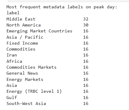
This metadata decomposition turns a quantitative spike into a qualitative narrative. Instead of just knowing that supply disruption coverage increased, we can see that it was driven by, for example, Middle East crude oil production stories — which immediately suggests what the market may be reacting to.
Because tokens.resolve_story() now accepts a list of story IDs and returns a DataFrame with story_id, the bulk decomposition step becomes a single call rather than a manual loop over stories.
9. Extending the Approach
Everything demonstrated here for energy supply disruptions is a pattern, not a one-off. The same methodology applies to any domain where Reuters News provides structured classification:
- Geopolitical risk: Sector + conflict/sanctions topic codes + geography
- Central bank policy: Topic codes for monetary policy + named entity codes for specific banks
- ESG events: Environmental or governance topic codes + sector + geography
- M&A activity: Deal/transaction topic codes + sector + named entities
In each case, the workflow is the same:
- Define the signal as a combination of structured metadata dimensions
- Retrieve stories matching the intersection
- Measure the signal over time
- Contextualize spikes using metadata decomposition
- Combine with other data for deeper analysis
The structured metadata transforms news from a reading experience into an analytical building block — something that can be defined precisely, measured consistently, and integrated into broader workflows.
Summary: Keyword searches match language. Structured metadata matches meaning. By defining a supply disruption signal as an intersection of sector, topic, and geographic classification codes — rather than a pattern of words — we get a cleaner, more complete, and more repeatable view of what's happening in energy markets. That signal can then be measured over time and combined with other market data to support analytical workflows that go well beyond reading headlines.
- Register or Log in to applaud this article
- Let the author know how much this article helped you
