Author

Forecasting USA GDP via Expenditure Approach and the Holt-Winters Model
Gross Domestic Product (GDP) is often thought of and calculated with an Expenditure Approach such that
GDP=C+I+G+(X−M)
where C = Consumption, I = Investment, G = Government Spending, & (X–M) = Net Exports.
The United States of America( USA)'s GDP (US GDP) is released quarterly by the Bureau of Economic Analysis, U.S. Department of Commerce. The only aforementioned component of US GDP released on a monthly basis is C, USA's Consumption Data. Monthly figures of GDP figures are thus not available, and estimating such values have proven of interest in academia (Mitchell, Smith, Weale, Wright, and Salazar (2005)) and in practice.
In this article, we will attempt to compute monthly US GDP estimates via the Holt-Winters (HW) method (resources on the HW model can be found here and - for academics - here). We then put ourselves in the shoes of an analyst who only has quarterly GDP component data (C, I, G or (X-M)). She/He uses the latest quarterly releases of GDP component data which spans from 2007 (in this study) to last quarter (last month at the earliest). She/He then uses the Holt-Winters method model to compute a forecast for the current period (month).
Accurate monthly GDP figures can be of great use in macroeconomic models going forward.
Development Tools & Resources
The example code demonstrating the use case is based on the following development tools and resources:
- Refinitiv's DataStream Web Services (DSWS): Access to DataStream data. A DataStream or Refinitiv Workspace IDentification (ID) will be needed to run the code below.
- Python Environment: Tested with Python 3.7
- Packages: DatastreamDSWS, Numpy, Pandas, statsmodel, scipy and Matplotlib. The Python built in modules os, warnings, statistics, datetime and dateutil are also required.
Import libraries
We need to gather our data. Since Refinitiv's DataStream Web Services (DSWS) allows for access to the most accurate and wholesome end-of-day (EOD) economic database (DB), naturally it is more than appropriate. We can access DSWS via the Python library "DatastreamDSWS" that can be installed simply by using pip installpip install.
Make sure to entre correct DataStream credentials
The following are Python-built-in module/library, therefore it does not have a specific version number.
statistics, numpy, scipy and statsmodels are needed for datasets' statistical and mathematical manipulations.
Make sure to have the latest version of statsmodels, versions before 10 tend not to be able to deal with numbers as large as the ones we are dealing with.
pandas will be needed to manipulate data sets
matplotlib is needed to plot graphs of all kinds
Setup Original Functions
Setup data sets
The cell below defines a function that translates DataStream data into a shape we can work with: a Pandas Dafaframe normalised to the 1st of the month that it was collected in.
The cell below defines a function that appends our monthly data-frame with chosen data
Setup plot functions
The cell below defines a function to plot data on one y axis.
The cell below defines a function to plot data regressed on time.
Setup Statistics Tools
The cell below defines a function that creates and displays a table of statistics for all vectors (columns) within any two specified datasets.
Monthly Data
U.S.A.'s Consumption Data
Quarterly Data
G.D.P. Component Sum


U.S.A.'s G.D.P.
To check our model, we can use 'United States, National Product Account, Gross Domestic Product, Overall, Total, Current Prices, AR, SA, USD'.
Data Résumé
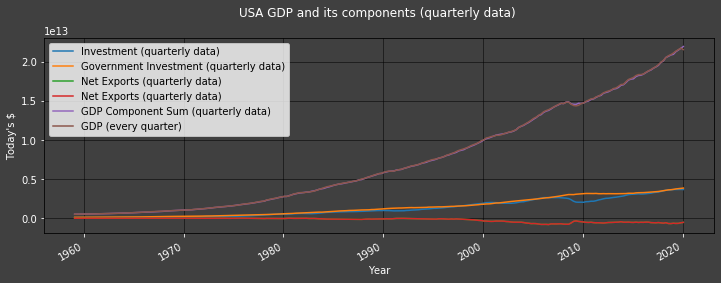
Note that the GDP and GDP Component Sum datapoints align so well that they are indistinguishable in the graph above
| Consumption (monthly data) | Investment (quarterly data) | Investment (monthly step data) | Government Investment (quarterly data) | Government Investment (monthly step data) | Net Exports (quarterly data) | Net Exports (monthly step data) | GDP Component Sum (quarterly data) | GDP Component Sum (monthly step data) | GDP (every quarter) | GDP (monthly step data) | |
|---|---|---|---|---|---|---|---|---|---|---|---|
| 1950-02-01 | NaN | 4.472500e+10 | 4.472500e+10 | 4.895600e+10 | 4.895600e+10 | 2.203000e+09 | 2.203000e+09 | NaN | NaN | 2.808280e+11 | 2.808280e+11 |
| 1950-03-01 | NaN | NaN | 4.472500e+10 | NaN | 4.895600e+10 | NaN | 2.203000e+09 | NaN | NaN | NaN | 2.808280e+11 |
| 1950-04-01 | NaN | NaN | 4.472500e+10 | NaN | 4.895600e+10 | NaN | 2.203000e+09 | NaN | NaN | NaN | 2.808280e+11 |
| 1950-05-01 | NaN | 4.945800e+10 | 4.945800e+10 | 4.964300e+10 | 4.964300e+10 | 1.643000e+09 | 1.643000e+09 | NaN | NaN | 2.903830e+11 | 2.903830e+11 |
| 1950-06-01 | NaN | NaN | 4.945800e+10 | NaN | 4.964300e+10 | NaN | 1.643000e+09 | NaN | NaN | NaN | 2.903830e+11 |
| ... | ... | ... | ... | ... | ... | ... | ... | ... | ... | ... | ... |
| 2020-03-01 | 1.390677e+13 | NaN | 3.669469e+12 | NaN | 3.850661e+12 | NaN | -5.261540e+11 | NaN | 2.090074e+13 | NaN | 2.153491e+13 |
| 2020-04-01 | 1.201326e+13 | NaN | 3.669469e+12 | NaN | 3.850661e+12 | NaN | -5.261540e+11 | NaN | 1.900724e+13 | NaN | 2.153491e+13 |
| 2020-05-01 | NaN | NaN | NaN | NaN | NaN | NaN | NaN | NaN | NaN | NaN | NaN |
| 2020-06-01 | NaN | NaN | NaN | NaN | NaN | NaN | NaN | NaN | NaN | NaN | NaN |
| 2020-07-01 | NaN | NaN | NaN | NaN | NaN | NaN | NaN | NaN | NaN | NaN | NaN |
Holt-Winters (HW) method
Creating a function to streamline use of Holt-Winters model
Example of our use of the Holt-Winters model: Investment data
The Holt_Winders_Method function may be a bit daunting, so let’s look at it step by step. 1st, this is our Investment data:
Notice that this is 'monthly step data', i.e. we only collected quarterly data and filled in the blanks (every month in-between each published value) with the latest published value available.
2nd: We apply the Holt-Winters model to this data to compute estimates:
Getting warnings at this stage is expected due to computational limitations, they should not impede our study.
U.S.A.'s Investments' Estimates using the HW method

| Mean of Absolute Values | |
|---|---|
| Investment forecasts (monthly step data) | 3.66466e+12 |
| Investment fitted values' real errors (monthly step data) | 7.88281e+09 |
U.S.A.'s Government Investment using the HW method

U.S.A.'s Net Exports of Goods and Services using the HW method
df with Holt-Winters estimates
Remember that certain measurements were not published all the way back in 1950; we only went all the way back to show how far one may try and go. As a result, certain rows in ' df ' will have a few 'NaN's at the start. Remember also that some variables (rows) are published only every quarter (quarterly data), so they ought to have 'NaN' values inter-quarter. These 'NaN's are expected and handled.
| Consumption (monthly data) | Investment (quarterly data) | Investment (monthly step data) | Government Investment (quarterly data) | Government Investment (monthly step data) | Net Exports (quarterly data) | Net Exports (monthly step data) | GDP Component Sum (quarterly data) | GDP Component Sum (monthly step data) | GDP (every quarter) | GDP (monthly step data) | Investment fitted values (monthly step data) | Investment forecasts (monthly step data) | Investment fitted values' real errors (monthly step data) | Government Investment fitted values (monthly step data) | Government Investment forecasts (monthly step data) | Government Investment fitted values' real errors (monthly step data) | Net Exports (monthly step data) positive | Net Exports fitted values (monthly step data) | Net Exports forecasts (monthly step data) | Net Exports fitted values' real errors (monthly step data) | |
|---|---|---|---|---|---|---|---|---|---|---|---|---|---|---|---|---|---|---|---|---|---|
| 1950-02-01 | NaN | 4.472500e+10 | 4.472500e+10 | 4.895600e+10 | 4.895600e+10 | 2.203000e+09 | 2.203000e+09 | NaN | NaN | 2.808280e+11 | 2.808280e+11 | 4.473305e+10 | NaN | 8.046422e+06 | 4.874360e+10 | NaN | -2.124022e+08 | 8.078330e+11 | 2.203000e+09 | NaN | 6.103516e-04 |
| 1950-03-01 | NaN | NaN | 4.472500e+10 | NaN | 4.895600e+10 | NaN | 2.203000e+09 | NaN | NaN | NaN | 2.808280e+11 | 4.473402e+10 | NaN | 9.016674e+06 | 4.902633e+10 | NaN | 7.033441e+07 | 8.078330e+11 | 2.203000e+09 | NaN | 6.103516e-04 |
| 1950-04-01 | NaN | NaN | 4.472500e+10 | NaN | 4.895600e+10 | NaN | 2.203000e+09 | NaN | NaN | NaN | 2.808280e+11 | 4.473169e+10 | NaN | 6.693394e+06 | 4.914832e+10 | NaN | 1.923165e+08 | 8.078330e+11 | 2.203000e+09 | NaN | 6.103516e-04 |
| 1950-05-01 | NaN | 4.945800e+10 | 4.945800e+10 | 4.964300e+10 | 4.964300e+10 | 1.643000e+09 | 1.643000e+09 | NaN | NaN | 2.903830e+11 | 2.903830e+11 | 4.472868e+10 | NaN | -4.729321e+09 | 4.917447e+10 | NaN | -4.685265e+08 | 8.072730e+11 | 2.203000e+09 | NaN | 5.600000e+08 |
| 1950-06-01 | NaN | NaN | 4.945800e+10 | NaN | 4.964300e+10 | NaN | 1.643000e+09 | NaN | NaN | NaN | 2.903830e+11 | 4.835530e+10 | NaN | -1.102705e+09 | 4.960638e+10 | NaN | -3.662454e+07 | 8.072730e+11 | 1.677304e+09 | NaN | 3.430377e+07 |
| ... | ... | ... | ... | ... | ... | ... | ... | ... | ... | ... | ... | ... | ... | ... | ... | ... | ... | ... | ... | ... | ... |
| 2020-03-01 | 1.390677e+13 | NaN | 3.669469e+12 | NaN | 3.850661e+12 | NaN | -5.261540e+11 | NaN | 2.090074e+13 | NaN | 2.153491e+13 | 3.672520e+12 | NaN | 3.050993e+09 | 3.853500e+12 | NaN | 2.839156e+09 | 2.794760e+11 | -5.253440e+11 | NaN | 8.099583e+08 |
| 2020-04-01 | 1.201326e+13 | NaN | 3.669469e+12 | NaN | 3.850661e+12 | NaN | -5.261540e+11 | NaN | 1.900724e+13 | NaN | 2.153491e+13 | 3.668037e+12 | NaN | -1.432291e+09 | 3.864030e+12 | NaN | 1.336876e+10 | 2.794760e+11 | -5.180397e+11 | NaN | 8.114276e+09 |
| 2020-05-01 | NaN | NaN | NaN | NaN | NaN | NaN | NaN | NaN | NaN | NaN | NaN | NaN | 3.666572e+12 | NaN | NaN | 3.866814e+12 | NaN | NaN | NaN | -5.202101e+11 | NaN |
| 2020-06-01 | NaN | NaN | NaN | NaN | NaN | NaN | NaN | NaN | NaN | NaN | NaN | NaN | 3.664588e+12 | NaN | NaN | 3.876213e+12 | NaN | NaN | NaN | -5.175651e+11 | NaN |
| 2020-07-01 | NaN | NaN | NaN | NaN | NaN | NaN | NaN | NaN | NaN | NaN | NaN | NaN | 3.662814e+12 | NaN | NaN | 3.885343e+12 | NaN | NaN | NaN | -5.157501e+11 | NaN |
Back-testing our Method
The Python function defined in the cell below returns the In-Sample Recursive Prediction values of ' data ' using the Holt-Winters exponential smoother Plus it then provides forecasts for One Out-Of-Sample period (thus the acronym 'ISRPHWPOOOF'):
We will back-test our models from January 2007
Back-testing our Method with Investment data

In the graph above, we put ourselves in the shoes of an analyst who only has quarterly Investment data. She/He uses the latest quarterly releases of Investment data which spans from 1950 (in our examlpe) to last quarter (last month at the earliest). She/He then uses the HW model to compute a forecast for the current period (month) - in yellow in the graph above.
Back-testing our Method with Government Investment data

Back-testing our Method with Net Exports data

G.D.P. Monthly Estimates

Conclusion
It is possible to estimate monthly US GDP figures using the HW model to a good degree of accuracy. The final forecast even anticipated the fall in GDP caused by COVID-19 (in 2020) before official figures were released. Such estimates can not only be done via an Expenditure Approach but also an Income Approach; a mixture of the two would be an interesting study.
Note that it is possible to use this method to compute future monthly GDP forecasts.
df
| Consumption (monthly data) | Investment (quarterly data) | Investment (monthly step data) | Government Investment (quarterly data) | Government Investment (monthly step data) | Net Exports (quarterly data) | Net Exports (monthly step data) | GDP Component Sum (quarterly data) | GDP Component Sum (monthly step data) | GDP (every quarter) | GDP (monthly step data) | Investment fitted values (monthly step data) | Investment forecasts (monthly step data) | Investment fitted values' real errors (monthly step data) | Government Investment fitted values (monthly step data) | Government Investment forecasts (monthly step data) | Government Investment fitted values' real errors (monthly step data) | Net Exports (monthly step data) positive | Net Exports fitted values (monthly step data) | Net Exports forecasts (monthly step data) | Net Exports fitted values' real errors (monthly step data) | Investment model in sample plus one forecast | Investment model in sample plus one forecast error | Government Investment model in sample plus one forecast | Government Investment model in sample plus one forecast error | Net Exports model in sample plus one forecast | Net Exports model in sample plus one forecast error | Computed GDP | |
|---|---|---|---|---|---|---|---|---|---|---|---|---|---|---|---|---|---|---|---|---|---|---|---|---|---|---|---|---|
| 1950-02-01 | NaN | 4.472500e+10 | 4.472500e+10 | 4.895600e+10 | 4.895600e+10 | 2.203000e+09 | 2.203000e+09 | NaN | NaN | 2.808280e+11 | 2.808280e+11 | 4.473305e+10 | NaN | 8.046422e+06 | 4.874360e+10 | NaN | -2.124022e+08 | 8.078330e+11 | 2.203000e+09 | NaN | 6.103516e-04 | NaN | NaN | NaN | NaN | NaN | NaN | NaN |
| 1950-03-01 | NaN | NaN | 4.472500e+10 | NaN | 4.895600e+10 | NaN | 2.203000e+09 | NaN | NaN | NaN | 2.808280e+11 | 4.473402e+10 | NaN | 9.016674e+06 | 4.902633e+10 | NaN | 7.033441e+07 | 8.078330e+11 | 2.203000e+09 | NaN | 6.103516e-04 | NaN | NaN | NaN | NaN | NaN | NaN | NaN |
| 1950-04-01 | NaN | NaN | 4.472500e+10 | NaN | 4.895600e+10 | NaN | 2.203000e+09 | NaN | NaN | NaN | 2.808280e+11 | 4.473169e+10 | NaN | 6.693394e+06 | 4.914832e+10 | NaN | 1.923165e+08 | 8.078330e+11 | 2.203000e+09 | NaN | 6.103516e-04 | NaN | NaN | NaN | NaN | NaN | NaN | NaN |
| 1950-05-01 | NaN | 4.945800e+10 | 4.945800e+10 | 4.964300e+10 | 4.964300e+10 | 1.643000e+09 | 1.643000e+09 | NaN | NaN | 2.903830e+11 | 2.903830e+11 | 4.472868e+10 | NaN | -4.729321e+09 | 4.917447e+10 | NaN | -4.685265e+08 | 8.072730e+11 | 2.203000e+09 | NaN | 5.600000e+08 | NaN | NaN | NaN | NaN | NaN | NaN | NaN |
| 1950-06-01 | NaN | NaN | 4.945800e+10 | NaN | 4.964300e+10 | NaN | 1.643000e+09 | NaN | NaN | NaN | 2.903830e+11 | 4.835530e+10 | NaN | -1.102705e+09 | 4.960638e+10 | NaN | -3.662454e+07 | 8.072730e+11 | 1.677304e+09 | NaN | 3.430377e+07 | NaN | NaN | NaN | NaN | NaN | NaN | NaN |
| ... | ... | ... | ... | ... | ... | ... | ... | ... | ... | ... | ... | ... | ... | ... | ... | ... | ... | ... | ... | ... | ... | ... | ... | ... | ... | ... | ... | ... |
| 2020-03-01 | 1.390677e+13 | NaN | 3.669469e+12 | NaN | 3.850661e+12 | NaN | -5.261540e+11 | NaN | 2.090074e+13 | NaN | 2.153491e+13 | 3.672520e+12 | NaN | 3.050993e+09 | 3.853500e+12 | NaN | 2.839156e+09 | 2.794760e+11 | -5.253440e+11 | NaN | 8.099583e+08 | 3.672520e+12 | -3.051000e+09 | 3.853505e+12 | -2.844000e+09 | -5.252940e+11 | -8.600000e+08 | 2.090750e+13 |
| 2020-04-01 | 1.201326e+13 | NaN | 3.669469e+12 | NaN | 3.850661e+12 | NaN | -5.261540e+11 | NaN | 1.900724e+13 | NaN | 2.153491e+13 | 3.668037e+12 | NaN | -1.432291e+09 | 3.864030e+12 | NaN | 1.336876e+10 | 2.794760e+11 | -5.180397e+11 | NaN | 8.114276e+09 | 3.668037e+12 | 1.432000e+09 | 3.864037e+12 | -1.337600e+10 | -5.179633e+11 | -8.190700e+09 | 1.902737e+13 |
| 2020-05-01 | NaN | NaN | NaN | NaN | NaN | NaN | NaN | NaN | NaN | NaN | NaN | NaN | 3.666572e+12 | NaN | NaN | 3.866814e+12 | NaN | NaN | NaN | -5.202101e+11 | NaN | 3.666572e+12 | NaN | 3.866814e+12 | NaN | -5.202101e+11 | NaN | NaN |
| 2020-06-01 | NaN | NaN | NaN | NaN | NaN | NaN | NaN | NaN | NaN | NaN | NaN | NaN | 3.664588e+12 | NaN | NaN | 3.876213e+12 | NaN | NaN | NaN | -5.175651e+11 | NaN | NaN | NaN | NaN | NaN | NaN | NaN | NaN |
| 2020-07-01 | NaN | NaN | NaN | NaN | NaN | NaN | NaN | NaN | NaN | NaN | NaN | NaN | 3.662814e+12 | NaN | NaN | 3.885343e+12 | NaN | NaN | NaN | -5.157501e+11 | NaN | NaN | NaN | NaN | NaN | NaN | NaN | NaN |
References:
Mitchell, Smith, Weale, Wright, and Salazar (2005): James Mitchell, Richard J. Smith, Martin R. Weale, Stephen Wright, Eduardo L. Salazar, An Indicator of Monthly GDP and an Early Estimate of Quarterly GDP Growth, The Economic Journal, Volume 115, Issue 501, February 2005, Pages F108–F129, https://doi.org/10.1111/j.0013-0133.2005.00974.x