Purpose
This tutorial is the third in a series on Tick History data inside Google BigQuery.
The preceding tutorial explained how to retrieve tick data, and filter it, using SQL.
This tutorial introduces actual analytics on the data.
The following tutorial will go further, giving you tips on how to optimize queries.
For your convenience, a set of sample queries is available in a downloadable file.
Easy analytics using SQL functions
There are many use cases for analytics based on tick history data, that cover typical needs of the front and middle office; for examples, refer to the Tick History in Google BigQuery article.
As a first example, let us analyse quotes. We shall calculate several statistics. Among these, the number of quotes is an indication of liquidity, whereas large swings in bid and ask prices or large percentage spread draw attention to instruments that could deliver interesting trading opportunities.
We perform the analysis using SQL, which has a set of built-in functions to count items, find minimum and maximum values, perform calculations, compare strings, and much more. We use these to enhance our query results. If you are a seasoned SQL programmer, you can also create your own User Defined Functions (UDF).
Quote statistics
The following query, based on quotes, analyses all available instruments on the London Stock Exchange. For each one it calculates a set of statistics. It also filters out irrelevant quotes based on qualifiers.
We sort the results by the number of quotes, to focus on finding liquidity.
#StandardSQL
SELECT
RIC,
COUNT(RIC) AS QuotesCount,
MIN(Bid_Price) AS MinBid,
MAX(Bid_Price) AS MaxBid,
MIN(Ask_Price) AS MinAsk,
MAX(Ask_Price) AS MaxAsk,
ROUND(SAFE_DIVIDE(100*(MAX(Bid_Price)-MIN(Bid_Price)),AVG(Bid_Price)),3) AS DeltaBidPercent,
ROUND(SAFE_DIVIDE(100*(MAX(Ask_Price)-MIN(Ask_Price)),AVG(Ask_Price)),3) AS DeltaAskPercent,
ROUND(AVG(Bid_Price),3) AS AvgBid,
ROUND(AVG(Ask_Price),3) AS AvgAsk,
ROUND(AVG(Ask_Price-Bid_Price),5) AS AverageSpread,
ROUND(AVG(SAFE_DIVIDE(100*(Ask_Price-Bid_Price),(Ask_Price+Bid_Price)/2)),5) AS AverageSpreadPercent
FROM
`dbd-sdlc-prod.LSE_NORMALISED.LSE_NORMALISED`
WHERE
RIC LIKE "%.L%"
AND (Date_Time BETWEEN TIMESTAMP('2019-09-04 00:00:00.000000') AND
TIMESTAMP('2019-09-04 23:59:59.999999'))
AND Type="Quote"
AND ((Bid_Price IS NOT NULL AND Bid_Size IS NOT NULL) OR
(Ask_Price IS NOT NULL AND Ask_Size IS NOT NULL))
AND NOT (Qualifiers LIKE 'M[IMB_SIDE]')
AND NOT (Qualifiers LIKE 'M[ASK_TONE]')
AND NOT (Qualifiers LIKE 'M[BID_TONE]')
AND NOT (Qualifiers LIKE '[BID_TONE];[ASK_TONE]')
AND NOT (Qualifiers LIKE 'A[BID_TONE];A[ASK_TONE]')
GROUP BY
RIC
ORDER BY
QuotesCount DESC
Here is the result:
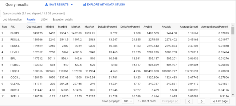
Note: NORMALISED data is level 1 data, the bid and ask prices are always the best bid and ask. For a more detailed view of the offers, we could have used NORMALISEDLL2 (market depth) data, which delivers a view of the top of the order book.
As you can see, this is quite powerful: all ticks for the full universe of LSE instruments for an entire day (12GB of data) were analysed in approximately 3 seconds to deliver 11 different calculated values for each of the 5600 instruments !
Trade statistics
Let us now see another example, based on trades, again for all instruments on the LSE. For each one it calculates the number of trades, the total traded volume, the minimum and maximum price, the price variation, and a few trade benchmarks such as VWAP, average price and volume. It also filters out irrelevant trades based on qualifiers.
We sort the results by the total volume, to focus on high trading volume instruments:
#standardSQL
SELECT
RIC,
ROUND(SAFE_DIVIDE(SUM(Volume*Price),SUM(Volume)),3) AS VWAP,
COUNT(RIC) AS TradesCount,
SUM(Volume) AS TotalVolume,
ROUND(AVG(Volume),0) AS AvgTradeVolume,
MIN(Price) AS MinPrice,
MAX(Price) AS MaxPrice,
ROUND(SAFE_DIVIDE(100*(MAX(Price)-MIN(Price)),AVG(Price)),3) AS DeltaPricePercent,
ROUND(AVG(Price),3) AS AvgPrice
FROM
`dbd-sdlc-prod.LSE_NORMALISED.LSE_NORMALISED`
WHERE
RIC LIKE "%.L%"
AND (Date_Time BETWEEN TIMESTAMP('2019-09-04 00:00:00.000000') AND
TIMESTAMP('2019-09-04 23:59:59.999999'))
AND Type="Trade"
AND Volume >0
AND Price >0
AND NOT (Qualifiers LIKE 'Off Book Trades%')
AND NOT (Qualifiers LIKE '%Previous Day Trade%')
AND NOT (Qualifiers LIKE '%CLS%')
AND NOT (Qualifiers LIKE 'U[ACT_FLAG1];U[CONDCODE_1]%')
AND NOT (Qualifiers LIKE '46---A---P----[MMT_CLASS]')
AND NOT (Qualifiers LIKE '46-1-A---P----[MMT_CLASS]')
AND NOT (Qualifiers LIKE '47---A---J----[MMT_CLASS]')
AND NOT (Qualifiers LIKE '47---A---P----[MMT_CLASS]')
AND NOT (Qualifiers LIKE '%Auction%')
GROUP BY
RIC
ORDER BY
TotalVolume DESC
Here is the result:
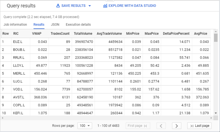
If you closely examined the quote and trade analytics code we have just seen, you might have noticed that the code was not written in an optimal manner: the maximum and minimum values were calculated in two different places, thus duplicating some of the effort. The next tutorial will come back to this topic, with a more efficient solution.
Market depth statistics
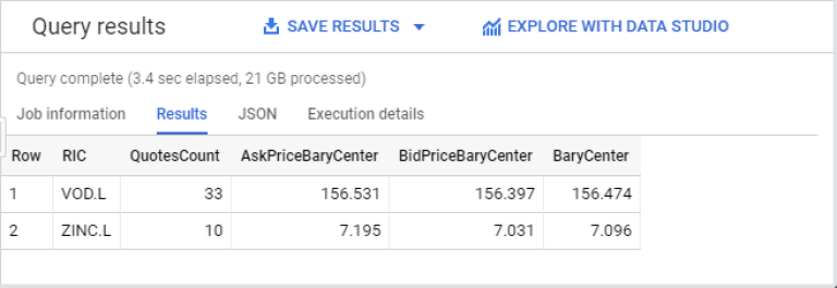
Let us see a final example, based on market depth data. We shall calculate a set of barycenter values. A barycenter is a mean weighted mean value. Here is the formula:
- Bid Barycenter = sum (bid vol * bid price) / sum (bid vol)
- Ask Barycenter = sum (ask vol * ask price) / sum (ask vol)
- Barycenter = (sum (bid vol * bid price) + sum (ask vol * ask price)) / (sum (bid vol) + sum (ask vol))
And here is the code:
#standardSQL
WITH
RAWSTATS AS(
SELECT
RIC,
COUNT(RIC) AS QuotesCount,
SUM((L1_BidPrice * L1_BidSize) + (L2_BidPrice * L2_BidSize) + (L3_BidPrice * L3_BidSize) + (L4_BidPrice * L4_BidSize) + (L5_BidPrice * L5_BidSize)) AS bidPriceVol,
SUM((L1_AskPrice * L1_AskSize) + (L2_AskPrice * L2_AskSize) + (L3_AskPrice * L3_AskSize) + (L4_AskPrice * L4_AskSize) + (L5_AskPrice * L5_AskSize)) AS askPriceVol,
SUM(L1_BidSize + L2_BidSize + L3_BidSize + L4_BidSize + L5_BidSize) AS bidVol,
SUM(L1_AskSize + L2_AskSize + L3_AskSize + L4_AskSize + L5_AskSize) as askVol
FROM
`dbd-sdlc-prod.LSE_NORMALISEDLL2.LSE_NORMALISEDLL2`
WHERE
(RIC LIKE "VOD.L" OR RIC LIKE "ZINC.L")
AND (Date_Time BETWEEN TIMESTAMP('2019-09-04 10:00:00.000000') AND
TIMESTAMP('2019-09-04 10:00:04.999999'))
AND (
((L1_BidPrice IS NOT NULL AND L1_BidSize IS NOT NULL) OR
(L1_AskPrice IS NOT NULL AND L1_AskSize IS NOT NULL))
OR ((L2_BidPrice IS NOT NULL AND L2_BidSize IS NOT NULL) OR
(L2_AskPrice IS NOT NULL AND L2_AskSize IS NOT NULL))
OR ((L3_BidPrice IS NOT NULL AND L3_BidSize IS NOT NULL) OR
(L3_AskPrice IS NOT NULL AND L3_AskSize IS NOT NULL))
OR ((L4_BidPrice IS NOT NULL AND L4_BidSize IS NOT NULL) OR
(L4_AskPrice IS NOT NULL AND L4_AskSize IS NOT NULL))
OR ((L5_BidPrice IS NOT NULL AND L5_BidSize IS NOT NULL) OR
(L5_AskPrice IS NOT NULL AND L5_AskSize IS NOT NULL))
)
GROUP BY
RIC
)
SELECT
RIC,
QuotesCount,
ROUND(SAFE_DIVIDE(askPriceVol,askVol),3) AS AskPriceBaryCenter,
ROUND(SAFE_DIVIDE(bidPriceVol,bidVol),3) AS BidPriceBaryCenter,
ROUND(SAFE_DIVIDE(askPriceVol+bidPriceVol,askVol+bidVol),3) AS BaryCenter
FROM
RAWSTATS
ORDER BY
RIC
LIMIT
100000
Here is the result:
Trade execution comparison
As a final example, let us take a trade we executed on the 4th of September 2019 at 14:10:30, at a price of 157.4, and compare it to the market in the same minute, to see how well we performed.
Here is the code, inside which we must input our trade price:
#standardSQL
# Compare your trade execution with the market.
# Inputs: line 48 (your trade price), 18 & 43 (instrument), 19 & 44 (date time range).
WITH
RAWSTATS AS(
SELECT
SAFE_DIVIDE(SUM(Volume*Price),SUM(Volume)) AS VWAP,
COUNT(RIC) AS TradesCount,
SUM(Volume) AS TotalVolume,
AVG(Volume) AS AvgVolume,
MIN(Price) AS MinPrice,
MAX(Price) AS MaxPrice,
AVG(Price) AS AvgPrice
FROM
`dbd-sdlc-prod.LSE_NORMALISED.LSE_NORMALISED`
WHERE
RIC LIKE "VOD.L"
AND (Date_Time BETWEEN TIMESTAMP('2019-09-04 14:10:00.000000') AND
TIMESTAMP('2019-09-04 14:11:00.000000'))
AND Type="Trade"
AND Volume >0
AND Price >0
AND NOT (Qualifiers LIKE 'Off Book Trades%')
AND NOT (Qualifiers LIKE '%Previous Day Trade%')
AND NOT (Qualifiers LIKE '%CLS%')
AND NOT (Qualifiers LIKE 'U[ACT_FLAG1];U[CONDCODE_1]%')
AND NOT (Qualifiers LIKE '46---A---P----[MMT_CLASS]')
AND NOT (Qualifiers LIKE '46-1-A---P----[MMT_CLASS]')
AND NOT (Qualifiers LIKE '47---A---J----[MMT_CLASS]')
AND NOT (Qualifiers LIKE '47---A---P----[MMT_CLASS]')
AND NOT (Qualifiers LIKE '%Auction%')
),
BETTERPRICE AS(
SELECT
COUNT(RIC) AS HigherPricedTradesCount,
SUM(Volume) AS TotalHigherPricedVolume,
SAFE_DIVIDE(SUM(Volume*Price),SUM(Volume)) AS HigherPricedVWAP
FROM
`LSE_NORMALISED.LSE_NORMALISED`
WHERE
RIC LIKE "VOD.L"
AND (Date_Time BETWEEN TIMESTAMP('2019-09-04 14:10:00.000000') AND
TIMESTAMP('2019-09-04 14:11:00.000000'))
AND Type="Trade"
AND Volume >0
AND Price>157.4
AND NOT (Qualifiers LIKE 'Off Book Trades%')
AND NOT (Qualifiers LIKE '%Previous Day Trade%')
AND NOT (Qualifiers LIKE '%CLS%')
AND NOT (Qualifiers LIKE '46---A---P----[MMT_CLASS]')
AND NOT (Qualifiers LIKE '46-1-A---P----[MMT_CLASS]')
AND NOT (Qualifiers LIKE '47---A---J----[MMT_CLASS]')
AND NOT (Qualifiers LIKE '47---A---P----[MMT_CLASS]')
AND NOT (Qualifiers LIKE '%Auction%')
)
SELECT
TradesCount,
TotalVolume,
ROUND(AvgVolume,0) AS AvgVolume,
MinPrice,
MaxPrice,
ROUND(AvgPrice,3) AS AvgPrice,
ROUND(VWAP,3) AS VWAP,
HigherPricedTradesCount,
ROUND(SAFE_DIVIDE(100*HigherPricedTradesCount,TradesCount),3) AS HigherPricedTradesPercent,
ROUND(TotalHigherPricedVolume,9) AS TotalHigherPricedVolume,
ROUND(HigherPricedVWAP,3) AS HigherPricedVWAP
FROM
RAWSTATS, BETTERPRICE
Here is the result, which shows how our trade is positioned compared to the market.
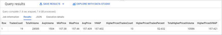
Note that this code, written in a fairly straightforward way to make it easy to understand, is a bit awkward, as the instrument and date time range must be input in 2 different places.
This puts us on the path to query optimization, which is the topic of the next tutorial.
Next step
We have seen how to use SQL functions to analyse data. Please proceed to the next tutorial that covers query optimization.