Download source code from |
 |
| Last update | January 2019 |
| Interpreter | Python 2.x/3.x |
Overview
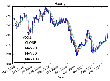
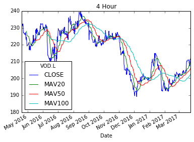
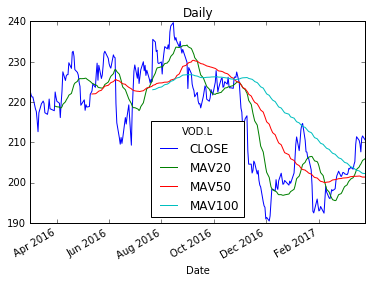
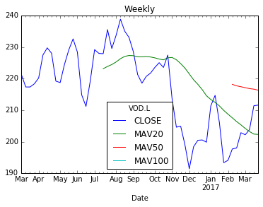
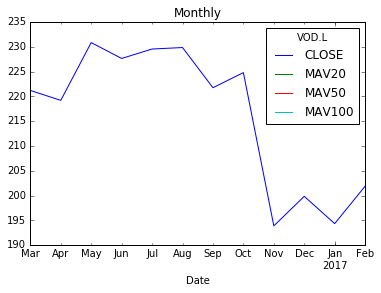
In this tutorial we will be downloading a timeseries of VOD.L (Vodafone) stockprice closes, for Hourly, Daily, Weekly and Monthly frequencies. We will then be creating a series of Simple Moving Averages (20, 50 & 100 period). I will also demonstrate how to resample the hourly timeseries to 4 Hour timeseries - using built-in functions of Pandas (this of course can be applied to other frequencies such as Minute - to generate 10 minute or 30 minute frequencies). Finally - I will plot these on a chart.
Before we start, let's make sure that:
- Eikon (version 4.0.36 or higher) or the Eikon Data APIs Proxy is up and running;
- Eikon API library is installed;
- You have created an App Key for this script.
If you have not yet done this, have a look at the quick start section for this API.
First off, lets load the libraries we will be using, eikon (for data retrieval), pandas (for dataframes) and matplotlib (for charting) - and we need to generate an App Key from Eikon and pass this to the App to allow download of data.
import eikon as ek #v0.14
import pandas as pd #v19
import matplotlib as plt
ek.set_app_key('your_app_key')
Next lets download some data and store the result in a few pandas dataframes - please note the use of the normalize=True parameter which you should use so that the dataframe is formatted correctly - this is important for both charting and calculation. We can also check we have downloaded data by looking at the tail (or head) of a dataframe.
Hourly = ek.get_timeseries(["VOD.L"], fields=["Close"], start_date = "2016-03-01", end_date = "2017-03-27",
interval="hour")
Daily = ek.get_timeseries(["VOD.L"], fields=["Close"], start_date = "2016-03-01", end_date = "2017-03-27",
interval="daily")
Weekly = ek.get_timeseries(["VOD.L"], fields=["Close"], start_date = "2016-03-01", end_date = "2017-03-27",
interval="weekly")
Monthly = ek.get_timeseries(["VOD.L"], fields=["Close"], start_date = "2016-03-01", end_date = "2017-03-27",
interval="monthly")
Hourly.tail()
| VOD.L | CLOSE |
|---|---|
| Date | |
| 2017-03-24 13:00:00 | 211.5500 |
| 2017-03-24 14:00:00 | 211.2245 |
| 2017-03-24 15:00:00 | 211.6000 |
| 2017-03-24 16:00:00 | 211.6500 |
| 2017-03-24 17:00:00 | 211.8000 |
Great! We now have data flowing into a dataframe which is automatically indexed with the date field (a datetiem object). Now I also want a 4 hour frequency frame, but I only have an hourly frequency - what to do? Thankfully pandas has some built-in functionality which allows us to resample the hourly data into (dis)aggregates thereof (known as downsampling) - in our case 4 hourly.
FourHour = Hourly.resample('4H').last().dropna()
FourHour.head()
| VOD.L | CLOSE |
|---|---|
| Date | |
| 2016-04-19 08:00:00 | 233.3160 |
| 2016-04-19 12:00:00 | 230.9000 |
| 2016-04-20 12:00:00 | 232.1500 |
| 2016-04-20 16:00:00 | 231.5856 |
| 2016-04-21 08:00:00 | 232.4500 |
Now that we have our resampled frame, lets generate some moving averages as new columns in each of the dataframes
framelist =['Hourly','FourHour','Daily','Weekly','Monthly']
for frame in framelist:
vars()[frame]['MAV20'] = vars()[frame]['CLOSE'].rolling(window=20).mean()
vars()[frame]['MAV50'] = vars()[frame]['CLOSE'].rolling(window=50).mean()
vars()[frame]['MAV100'] = vars()[frame]['CLOSE'].rolling(window=100).mean()
Hourly.tail()
| VOD.L | CLOSE | MAV20 | MAV50 | MAV100 |
|---|---|---|---|---|
| Date | ||||
| 2017-03-24 13:00:00 | 211.5500 | 209.283000 | 209.89438 | 207.322222 |
| 2017-03-24 14:00:00 | 211.2245 | 209.459225 | 209.93887 | 207.410967 |
| 2017-03-24 15:00:00 | 211.6000 | 209.636725 | 209.99087 | 207.503467 |
| 2017-03-24 16:00:00 | 211.6500 | 209.838225 | 210.02087 | 207.579967 |
| 2017-03-24 17:00:00 | 211.8000 | 210.060725 | 210.05287 | 207.664967 |
Voila! 3 shiny new moving averages in each frame. So, lets now plot these on a chart.
%matplotlib inline
Hourly.plot(title="Hourly")
FourHour.plot(title="4 Hour")
Daily.plot(title="Daily")
Weekly.plot(title="Weekly")
Monthly.plot(title="Monthly")
<matplotlib.axes._subplots.AxesSubplot at 0xab00550>
Appendix: Timeseries Output Formats
We have tried to design default outputs for the main different forms of request to make it more intuitive for downstream processing. Here I will go through the main request forms:
One Security, N Fields (one or more)
oneXN =ek.get_timeseries("VOD.L", fields='*', start_date = "2016-03-01", end_date = "2017-03-27",
interval="hour")
oneXN.tail()
| BARC.C | CLOSE |
|---|---|
| Date | |
| 2017-03-21 | 230.00 |
| 2017-03-22 | 224.55 |
| 2017-03-23 | 223.90 |
| 2017-03-24 | 226.95 |
| 2017-03-27 | 224.20 |
N Securities, N Fields
NxN = ek.get_timeseries(['BARC.L','VOD.L'], fields=["Open","High","Low","Close"], start_date = "2016-03-01", end_date = "2017-03-27",
interval="daily")
NxN.tail()
| Security | BARC.L | VOD.L | ||||||
|---|---|---|---|---|---|---|---|---|
| Field | CLOSE | HIGH | LOW | OPEN | CLOSE | HIGH | LOW | OPEN |
| Date | ||||||||
| 2017-03-21 | 212.200000 | 212.0 | 209.60 | 209.100 | NaN | NaN | NaN | NaN |
| 2017-03-22 | 210.212300 | 209.2 | 207.65 | 207.039 | NaN | NaN | NaN | NaN |
| 2017-03-23 | 211.850000 | 209.1 | 211.00 | 206.850 | NaN | NaN | NaN | NaN |
| 2017-03-24 | 211.850000 | 211.5 | 211.60 | 210.100 | NaN | NaN | NaN | NaN |
| 2017-03-27 | 211.291136 | 210.8 | 210.60 | 208.650 | NaN | NaN | NaN | NaN |
Normalisation
We also provide a normalize=True/False parameter which allows you to override our default output shapes and gives you a normalized output shape which you can then process as you wish - with four columns Date, Field, Security, Value.
norm = ek.get_timeseries(['BARC.L','VOD.L'], fields=["Open","High","Low","Close"], start_date = "2016-03-01", end_date = "2017-03-27",
interval="daily", normalize=True)
#norm.head()
norm.tail()
| Date | field | Security | Value | |
|---|---|---|---|---|
| 1083 | 2017-03-24 | CLOSE | VOD.L | 211.600000 |
| 1084 | 2017-03-27 | OPEN | VOD.L | 210.800000 |
| 1085 | 2017-03-27 | HIGH | VOD.L | 211.291136 |
| 1086 | 2017-03-27 | LOW | VOD.L | 208.650000 |
| 1087 | 2017-03-27 | CLOSE | VOD.L | 210.600000 |
Author: jason.ramchandani@refinitiv.com